Aaron Pickering

Despite what I think is the worst, tongue-twisting name in statistics, Heteroscedasticity is definitely a concept worth understanding.

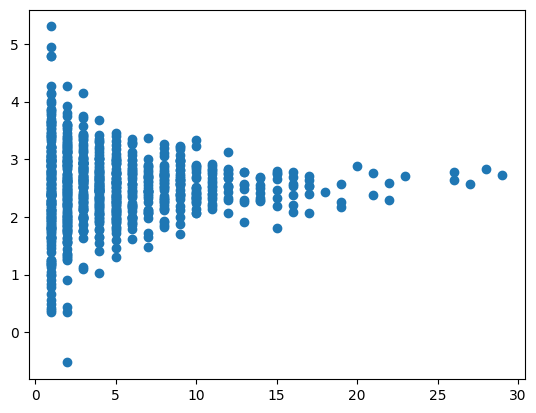
The idea itself is not particularly complicated – heteroscedasticity is when the variance isn’t constant across the range of a related variable. An example of heteroscedasticity is shown in the image below; the variance is larger closer to x=0 and smaller when x = 30.

It’s my experience that many Analysts, Data Scientists and Machine Learning engineers don’t think about the variance much when modelling. Truthfully, you might get away with that on occasion.

But on the occasions where it is important, you’ll need different processes and techniques to properly handle the data.

In this two part article, I’ll show you some techniques for working with heteroscedastic data. Today, I’ll start by discussing the simpler methods of transformations and basic linear models. Then in Part 2, I’ll expand the toolset towards more complicated problems.

Example based on Social Media Data

Heteroscedasticity is a real phenomenon that appears all the time in real life data. At Seenly, we handle a lot of social media data, much of it heteroscedastic. Inspired by this, I’ve created a simplified, simulated dataset for use in the examples that follow.

Consider the case of modelling LinkedIn data. On LinkedIn, users create content and hopefully, get engagements from their audience in the form of likes, comments and shares and new followers. The more people that follow you, the more engagement you are likely to get.

Suppose that we would like to understand and model the relationship between followers and the number of engagements generated by a single post. Stripping away some of the complexities (time of day, post quality, duration etc) to simplify the problem, the resulting chart might look something like the one below, where each blue dot represents a single post.

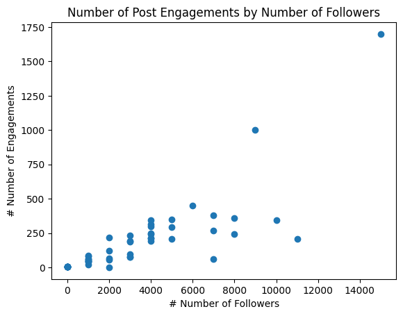
If you look closely, you can see that the variance is not consistent. People with fewer followers, receive fewer engagements and the observations are more tightly clustered i.e. lower variance. More followers brings more engagements but also a higher variance.

Consider what happens when I fit a standard linear model of the following form:

y = βx + c + ɛ

For this, I have used the Python package Statsmodels. The associated code is available via the Notebook on Github.

The results of the fit are shown in the images below.

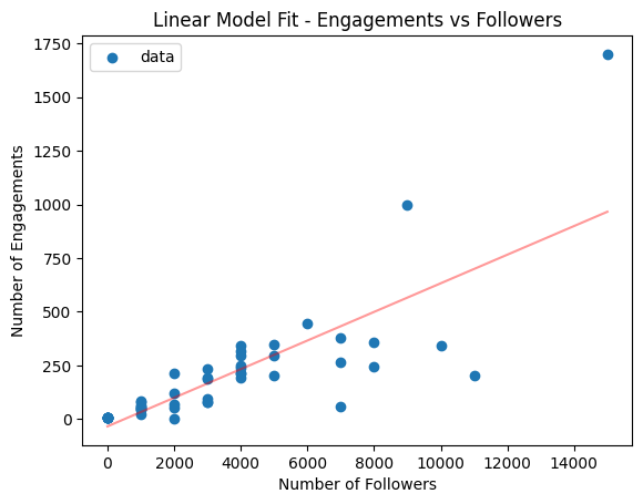
If you look at the fit in isolation (left image), it actually looks pretty good. The prediction goes down the middle of the data points so you could be forgiven for thinking that the job is done.

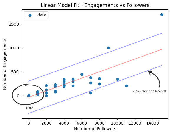
But, look at the image to the right where I’ve highlighted a couple of problems. Firstly, the linear model assumes constant variance so the 95% prediction interval (blue) is completely wrong. Its flat across the spectrum and doesn’t capture any variation. The high end isn’t wide enough and its way too conservative at the low end.

Secondly, take a closer look at the observations with fewer followers. It shoots a little low. The absolute error is still small but the model intercept skews low to compensate for the extra weight on observations with many followers. In percentage terms this error could be quite significant for some observations. Whether that’s a problem is debatable but it could be serious depending on the business context.

So, now that we’ve seen what can go wrong, how do we fix it?

Transformations

The easiest way to fix heteroscedasticity is to apply a transformation to the data. This will only work in very simple cases but its worth exploring first.

Power transformations are the most common way to do this. For example, if I take the log of both the ‘follower’ variable and the log of ‘engagements’ variable, we get the following plot.

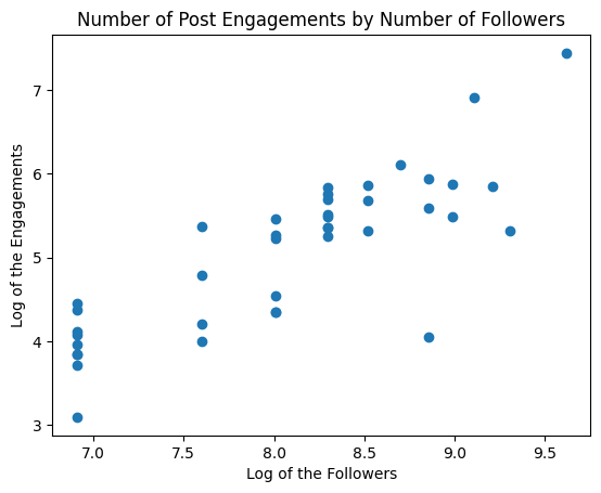
The variance has more or less stabilized. Problem solved.

Another transformation that is useful in practice is the square root. This can help fix heteroscedasticity for cases with where the y-variable is an average. This ‘funnel’ shape can be fixed by multiplying by square root of the x-axis variable.

Transformations are often very effective for simple problems, so explore your data and see if any of the common functions are suitable. If transformations don’t help, then a model based solution could be the logical next step.

Model based solutions

An alternative way to handle heteroscedasticity is to use a model based solution. These models can natively handle variations in the variance and are designed to do so.

In this section, we’ll look at two interesting models.

Firstly, Quantile Regression via Statsmodels and secondly, a Conditional Variance model using PyMC.

Quantile Regression

Quantile regression is a type of regression which aims to find one or more prediction quantiles, rather than the mean, as in the case of linear regression. The most common quantile is the median (0.5) but any quantile can be chosen and its this ability that helps us to model the heteroscedasticity.

Loosely, to train the model the positive and negative errors are balanced, with a weighting given by the quantile of interest. For example, if the quantile is 0.7 then 70% of the error distribution is on one side and 30% on the other.

More precisely, given a quantile of interest ‘q’, and prediction ‘y^p‘ and observations ‘y’, the loss is given by:

ℒ = argmax((q – 1)*(y – y^p), q*(y – y^p))

The model is not limited to a single quantile; any number can be optimised simultaneously subject to computational limitations.

Sklearn has an easy-to-follow implementation of Quantile regression. See how I have used it here on Github.

The plot below shows the predictions for our Quantile Regression model. Red is the median, purple the 25th and 75th percentiles and blue 95th.

• The variation in the variance has been correctly captured by the quantile regression
• The fit in the lower left corner is much better
• The uncertainty has been correctly modelled

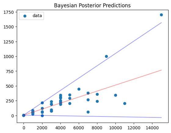
Conditional Variance Model

An alternative method, is to model the conditional variance directly.
Typically, when doing a linear regression model via Maximum Likelihood, we would assume a Gaussian distribution.

For this example, I have built the model using the Python library for Bayesian modelling, PyMC. You can see my code here on Github.

In the Maximum Likelihood (and Bayesian) context a standard linear model looks something like this:

y ~ 𝓝(μ, σ²)
μ = βx + c

Where the observations are drawn from a normal distribution 𝓝, with a mean μ and a standard deviation σ. In the standard case, only the mean is conditional upon our input x.

In our conditional variance model, standard deviation is also modelled as a linear function of the inputs. The formulation is therefore:

y ~ 𝓝(μ, σ²)
μ = βx + c
σ = γx + d

Bringing it back to our example, we are now modelling the mean relationship between the ‘followers’ and ‘engagements’ and the variance.

Plotting the results, we get the image below. The red line is the mean and the blue line is the 95% prediction interval. Just like the Quantile Regression, we can see that the:

• Variance has been correctly captured
• Fit in the lower left corner is much better
• Uncertainty has been correctly modelled

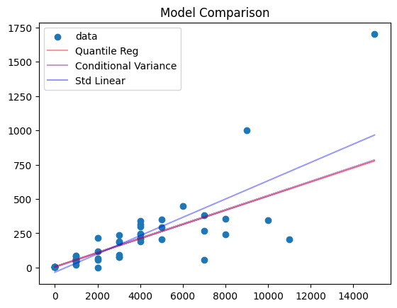
Model comparison

Finally, lets compare the results of our three models together. The plot below shows the prediction for the standard linear model, the Quantile Regression and the conditional variance model.

You can see that the Quantile Regression and the conditional variance model generate the same predictions. That’s because the errors are normally distributed and the median is the same as the mean in this particular case.

The standard linear model however, is significantly biased in comparison because it can’t capture the heteroscedasticity.

Summary

In this article, I’ve given a short introduction to heteroscedastic data and shown how you can handle it with transformations and model based approaches.

In particular, I’ve shown how we can use Quantile Regression and a conditional variance model to solve univariate, linear problems.

However, there are far more complicated problems out there. Non-linearity, multiple variables and larger datasets all make for greater challenges.

Therefore, in part 2, I’ll take a look at some methods to handle these new challenges. Stay tuned.

In the meantime, be on the look out for heteroscedasticity in your datasets!

---

Subscribe