Years ago, I wrote some code to help myself learn more about the inner workings of Bayesian methods. Back then, I found the exercise extremely helpful and so, having recently stumbled upon the code again, I decided to dust it off, clean it up and write it into a blog post for the benefit of anyone new to the topic. Let’s build a Bayesian regression from scratch.
Bayesian methods are especially powerful because they allow us to understand the uncertainty of our regression models in a very tangible way. They also allow us to incorporate existing knowledge into the model in a formalized form.
These benefits have led to an explosion of new Bayesian packages in recent years such as PyMC, BRMS and Pyro.
However, the inner workings of Bayesian methods can be a bit mysterious and therefore, building such a regression from scratch is a great exercise.
Lets get stuck in!
Data
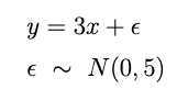
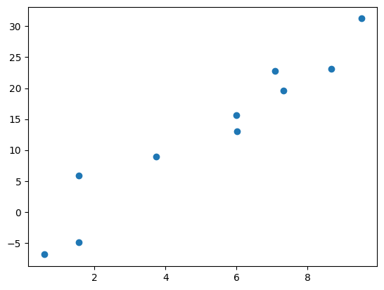
First lets generate some sample data according to the following formula below.
np.random.seed(42)
# Generate random draws for x and y
x = np.random.uniform(0, 10, 10)
y = 3 * x + np.random.normal(0, 5, 10)
y = 3x. This is about the easiest possible regression problem so its a great place to start understanding Bayesian regression. Our goal will be to build a model that predicts the line of best fit and learns the best value of the slope, uncertainty and all.
Bayes Rule
You’ve probably seen Bayes rule a million times so I won’t belabour the point. Basically, it defines how we can update our prior knowledge based on new data. If you haven’t heard of it, take quick detour of the wiki page.
However, for this post all you’ll need to know are some key terms.

In Bayesian regression we have:
- the Prior P(A) denotes our existing knowledge. If you don’t have any, just make it a constant – then it doesn’t affect anything and our model becomes a standard regression.
- the Likelihood P(B|A) is simply how well our model fits this data. If our fit is bad then its unlikely and we get a small number. If the fit is close, we get a big number.
- the Posterior P(A|B) – this is the distribution that we are trying to find. In this example, we are trying to retrieve slope of our regression line and we are trying to understand the uncertainty. The uncertainty is always represented by a distribution.
- P(B) is a normalizing constant. We can just ignore it because it doesn’t affect our parameter estimates.
Simply, to get the posterior we need to multiply likelihoods by the prior. Do that enough and we have a Bayesian model.
Maximum Likelihood Detour
Many people who’ve done some machine learning or statistics are familiar with the concept of the ‘Least Squares’ loss function i.e find a line of best fit that minimizes the distance between itself and the data points, squared. However, there is an alternative loss which is very important to for Bayesian methods.
Its called Maximum Likelihood – rather than finding the distance between the fit line and each point, we decide how likely the line is, given the points.
If the points are very far away from the line, that’s unlikely. If the points are close, its likely. We then try to maximize the likelihood, hence the name. Statistically, we use a specific function help us calculate how likely each point is. A Gaussian likelihood (normal distribution) is mathematically equivalent to least squares, so we’ll use that for this exercise.
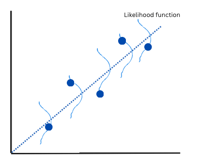
You can see in the image above, in light blue, I’ve overlaid little (badly drawn) Gaussian distributions over the fit line. If the point is closer to the centre, that’s likely. If its closer to the tails, its unlikely.
In the end, the line of best fit is just the most likely estimate, considering all the points.
And you can simply find the maximum by using scipy’s minimize function and multiplying by -1. The code to find the maximum likelihood is shown below.
# Likelihood function in Python
def likelihood(beta, sd):
    y_pred = beta * x
    res = y - y_pred
    l = norm.logpdf(res, loc=0, scale=sd).sum()
    return -l
result = minimize(likelihood, [1, 1], method="Nelder-Mead")
But remember, so far we’ve only found the maximum, we’re not yet Bayesian! For a Bayesian regression we need the full distribution of uncertainty.
Maximum Likelihood to Bayesian Regression
So, how do we go from the most likely estimate to a full Bayesian regression with uncertainty. Its just a matter of trying lots of different random fit lines and saving the results. If we look at enough fit lines and then check the results in aggregate, we’ll hopefully have a nice distribution showing our uncertainty across the parameter space.
There is one catch, however. We can’t just try every possible fit line. Maybe that would work, at a stretch, for a single parameter, but for 2, 3…….10? Trying every possible combination (or sampling in Bayesian terms) is impossible. We have to do it efficiently.
That’s where the Metropolis Hasting algorithm comes in.
MCMC Methods (Metropolis-Hastings)
Metropolis-Hastings is an algorithm for exploring the parameter space efficiently. Its definitely not the only sampling algorithm (for instance, modern libraries tend to use NUTS sampling) nor the most efficient, but it is foundational for Bayesian modelling.
You start the algorithm at some initial set of parameters and then the general idea is to jump around the search space, exploring all the possibilities, spending more time in the likely areas and less time in unlikely ones.
The algorithm proceeds as follows:
- Start with an initial sample from the target distribution.
- Create a proposal for a new sample. The proposal candidate is based on the current sample and is drawn from a ‘proposal distribution’.
- Calculate the likelihood of the proposal divided by the likelihood of current point. This ratio determines whether the proposed sample is accepted or rejected, with some randomness to encourage exploration. Higher ratios = higher acceptance rate.
- If the proposed sample is accepted, add it to the sequence of samples; otherwise, keep the current sample.
- Repeat 2-4 for ‘n’ iterations. A greater number of iterations tends to lead to better convergence.
Lets explore these steps in the code below.
# Define the likelihood functions
def prior_likelihood(params):
    return np.log(norm.pdf(params[0], 5, 3)) + np.log(norm.pdf(params[1], 10, 30))

def posterior_mh(beta, sd):
    return likelihood(beta, sd) + prior_likelihood([beta, sd])
# Set up the parameter matrix
parameters = np.empty((iterations, 5))
parameters[:, :] = np.nan
parameters[0, :] = [betas[0], sds[0], beta_p[0], sds_p[0], np.nan]

# Run the Metropolis-Hastings algorithm
for i in range(iterations-1):
    # 1. Calculate the posterior for the current iteration
    parameters[i, 4] = posterior_mh(parameters[i, 0], parameters[i, 1])

    # 2. Find a proposal point (check Github for the full code)
    proposals = jump_function(parameters[i, :2])

    # 3.1 Calculate the posterior for the proposal
    proposal_likelihood = posterior_mh(proposals['b_proposal'], proposals['sd_proposal'])

    #3.2
    acceptance_ratio = np.exp(proposal_likelihood - parameters[i, 4])

    # If the proposal likelihood is greater, always accept the proposal
    if acceptance_ratio > 1:
        parameters[i+1, :2] = proposals['b_proposal'], proposals['sd_proposal']
    else:
        # Otherwise, sometimes accept and sometimes explore
        p = np.random.uniform(0, 1)
        if p > (1 - acceptance_ratio):
            parameters[i+1, :2] = proposals['b_proposal'], proposals['sd_proposal']
        else:
            parameters[i+1, :2] = parameters[i, :2]
More info and full working code can be found here.
As you can see, the code is quite minimal. Despite that, we’ve built a very simple Bayesian regression algorithm from scratch. If you have a keen eye, perhaps you noticed that I added in some “prior knowledge” too.
Of course, its not scalable or efficient – use a proper package for Bayesian inference. However, hopefully I’ve given you some new intuition about how everything works under the hood.
Bayesian Regression Results
Here, the results themselves are not so important, rather their format.
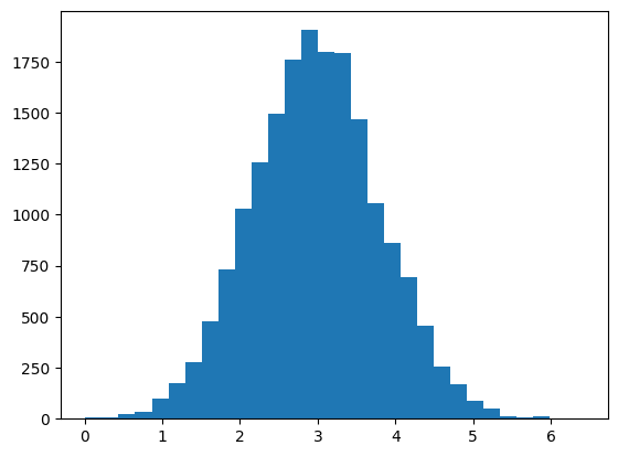
Firstly, we have obtained a posterior distribution for our parameter. You can see that the mean of this posterior distribution is roughly 3 as expected. But we can also see the possible range of the parameter helping us to understand the uncertainty. The posterior is a little thinner than it would be with the data alone – that’s the effect of the prior that I added. The prior shapes our view of the data – so only use when appropriate.
Posterior
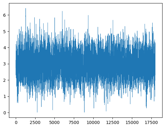
As well as the posterior, we also have generated a posterior chain (trace). The trace shows the path taken as the algorithm jumps around the distribution. If the algorithm has converged, the path will be roughly stationary (consistent mean and variance). That seems to be true in our case.
Posterior Chain
Summary
Back when I first learnt about Bayesian modelling, this coding exercise was very helpful in getting my head around all the concepts.
At the time, I found the concepts difficult to get my head around. Posteriors, sampling, likelihoods – all these things were alien to me. But the exercise of writing everything from scratch was extremely helpful.
Hopefully this same code has helped you get a little bit closer to these extremely useful methods.
Once again, to see full code please visit my Github page.

Leave a comment