Interrupted Time Series

When experimenting with something new, everyone has an opinion! Thats why it’s especially important to gather empirical evidence, to truly measure success. In this series of articles, I will explore a variety of techniques for experimentation, measurement and the gathering of evidence. Today’s article concerns one such fundamental technique – Interrupted Time Series analysis.

The Interrupted Time Series method is used to assess the impact of an intervention or event. The method itself is quite straightforward to implement, as you’ll see shortly. However, that simplicity comes with a number of caveats and assumptions that need satisfying.

Essentially, ITS is used to statistically measure the effect of an event on a time series dataset. The idea is to collect data before and after an intervention and then evaluate the magnitude and significance of any observed changes. It’s used in situations where you can’t run an randomised experiment or set up a proper control group. For example, consider a law or regulation that needs to be rolled out all at once, across an entire country. It would be unethical to apply the law selectively to different groups so techniques such as ITS are the best we can do.

Data

To make things fun, we’ll conduct our Interrupted Time Series analysis on some real data. In late 2021, Facebook changed their name to Meta. Let’s conduct an analysis before and after this “intervention” and see how search volume for the word meta was impacted.

A plot of the ‘meta’ Google search volume is shown below. The name change occurred in October 2021.

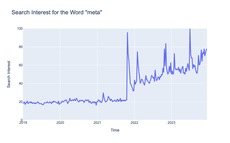
Note: Google Trends search volume is normalised between 0 and 100. These are relative search volumes, not absolute.

Of course, the word ‘meta’ was commonly used before Facebook/Meta came around. Thats why the plot shows search for the term before the name change.

At the same time, there’s no doubting that the announcement of the name change drastically increased public consciousness for the word ‘meta’. In the next sections we’ll analyze statistically how the search volume was impacted by this change.

Assumptions

Before we begin, there are some assumptions that need to be carefully considered. These assumptions determine whether Interrupted Time Series analysis is an appropriate tool.

Confounding

ITS attributes all of the pre and post name change difference to the name change itself. That’s a strong assumption!

If there were also other changes driving the search volume, the estimated impact of Facebook’s name change would be overestimated.

For example, what if during the same month as the name change, a book called ‘Meta’ climbed to the top of NY Times Best Seller list? Hidden confounders come up more often that most would like to believe and we should be conscious of them. Caution advised!

Linearity

For this analysis, we’ll be applying a segmented linear model in two sections. This is typical for a simple ITS analysis. However, its important to determine whether this actually make sense for your use case. Plot the data and see whether the linear assumption holds.

Target Distribution

It’s important to make sure that your model distribution matches the target distribution. In this case, I have chosen a Gaussian Distribution.

Many people would advocate for a statistical test e.g Shapiro-Wilk Test to determine a suitable distribution and I don’t entirely disagree. However, time series data can often deceive standard tests so be sure sure to use your eyeballs and get a feel for the data first.

As an example, when I plot a histogram of the target you see something very not-gaussian.

But thats largely because our time series consists of two different sections and a strong trend. If we control for the trend, we’ll Gaussian errors around a local mean. Proof can be found in the results below. Regardless, check for trends, skew and think about the data generating process and choose your distribution appropriately.

Consistent Variance

For simplicity, I will conduct the regression as if the variance were consistent pre and post intervention. This isn’t entirely true but experience tells me its unlikely to affect the outcome very much. If you would like to learn more about controlling for the changing variance, read more here.

Setup and Preprocessing

There are several ways to pre-process the data for this problem, each equally effective. The simplest method is to create two separate independent variables, one for pre-name change and one post-name change and then estimate the effects simultaneously with a regression model.

Firstly, we must identify the time of the name change. According to this source, Facebook announced the change officially on the 21st of October 2021. I’ve plot the before and after variable in orange below. Given there was some build up to the change, I’ve left September and October empty as a transition period.

Next, we create our two input variables. I have called these variables ‘t_pre’ and ‘t_post’ representing the time before the name change and the time after. These variables simply represent the number of weeks since 2018-12-30.

At this point, our data set is ready and we can begin to model!

Interrupted Time Series Model

We’ll use a regression model to estimate the following equation:

$\text{meta} = \beta_1 \cdot t_{\text{pre}} + \beta_2 \cdot t_{\text{post}} + \gamma_{\text{pre}} + \gamma_{\text{post}}$

Let’s break down the components:

meta: our target variable, the amount of google search for the word ‘meta’
$\beta_1$ : a coefficient determining the slope of the line before the intervention
$\beta_2$ : a coefficient determining the slope of the line after the intervention
$\gamma_{\text{pre}}$ : a term indicating the baseline amount of search before the intervention. An intercept.
$\gamma_{\text{post}}$ : a term indicating the additional amount of search gained immediately after the intervention.

For the code, I will use the Python package statsmodels, which has a convenient API for Linear Regression. Additionally, I have provided code for the Bayesian equivalent using Bambi and PyMC

Code: Frequentist Approach

The following code defines a linear regression model (OLS) with the formula as above. After the defining the formula, we fit the model and store the result.

import statsmodels.formula.api as smf
import pandas as pd

# Formula Definition
formula = 'meta ~ t_pre + t_post + 1 + intervention'

# Fit the linear mixed-effects model
model = smf.ols(formula, df.dropna())
result = model.fit()

Code: Bayesian Approach

Below is the equivalent code using the Bayesian framework. I’ve used default, uninformative priors so that the end results are the same either way. The Bayesian approach provides us additional uncertainty estimates which will be of use later on.

# Fit the Bayesian Linear model using Bambi (PyMC)
model = bmb.Model('meta ~ t_pre + t_post + 1 + intervention', dropna=True, data=df)
result = model.fit(draws=5000, chains=2)

Model Diagnostics

Before we look at the results we should check some diagnostics and make sure everything was specified correctly. Firstly, lets look at the fit:

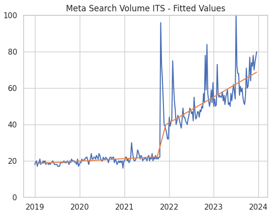
At first glance, the fit looks pretty good and captures the trend nicely.

Next, let’s look at the errors. As previously mentioned, OLS Linear Regression assumes Gaussian errors. As you can see below, the errors are roughly normally distributed as required with a couple of outliers.

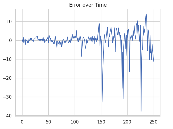
Finally, if we’ve modeled the trend correctly, the errors (residuals) shouldn’t be autocorrelated. That is, they shouldn’t be related in time.

The diagnostic plots below can help us determine whether this is the case. The plot on the left is a Partial Autocorrelation Function plot. It shows whether points in our time series errors are correlated with the values that came before them.

Largely, we’ve removed the autocorrelation but there is still some remaining at lag 1 and 2 i.e the current error is related to the previous error and the error before that.

The plot on the right shows the error over time. While the mean consistently hovers around zero there are some autocorrelated deviations, particularly at the end. These deviations are linked to the autocorrelation that we found in the PACF plot. Finally, the errors increase after the name change - we have heteroscedasticity.

Does this mean that our model is badly specified? Well, no, but its not perfect.

Statistician George Box once said ‘All models are wrong; some are useful‘, which applies here. Simply put, our strictly linear ITS model doesn’t perfectly capture the changes and movements over time.

However, the fit looks fine, the residuals are mostly Gaussian and we’ve removed the majority of the autocorrelation. This model is well specified and importantly, useful.

Results

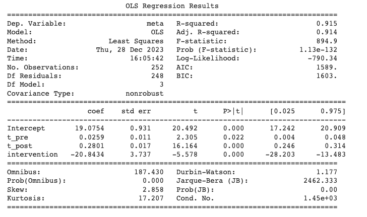
Above is the result summary of our Interrupted Time Series regression.

The key results are:

t_pre & t_post: The two numbers in the ‘coef’ column indicate the estimated size of the slopes before and after the intervention. The post intervention slope is just over 10 times greater than the pre intervention slope.
intercept and intervention: These terms correspond to the baselines in our above formula. ‘Intercept’ is the baseline level pre intervention. The second term is a little harder to interpret. Nominally, it represents the baseline post intervention, however the number is derived from the sum of all the slopes and intercept. To obtain the true value we need to calculate backwards using the code below. The final baseline values are 19 and 42 for pre and post respectively.

df['t_post'].unique()[1]*t_post + intervention + df['t_pre'].max()*t_pre + intercept

Simply put, we can see that that there has been significantly more search for the word ‘meta’ since Facebook changed their name.

As well as the coefficients themselves, included in the table are also several important diagnostic statistics. Most importantly, the column $P > |t|$ contains the respective p-values, which in this case are all significant.

Counterfactual

Exactly how much extra search was generated by the name change? To answer this question we need to create what is known as a ‘counterfactual’.

A counterfactual is a prediction of what would have happened without the intervention. Put simply, if Facebook didn’t change their name, how many people would be searching for the word ‘meta’ today

To answer that question, we can actually just use our existing model and create a prediction using the pre-intervention slope and intercept. The plot below shows the estimated counterfactual and contains a 97% confidence interval derived from the Bayesian regression.

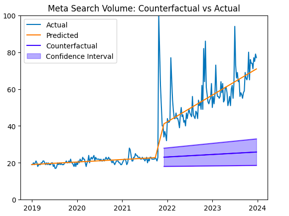
Even pessimistically, the name change had a strong and signficant impact on the amount of search for the word ‘meta’, completely as expected.

To calculate the actual impact, we simply subtract the counterfactual from what actually happened and count the difference.

Below is a plot showing the difference between the counterfactual and what actually happened.

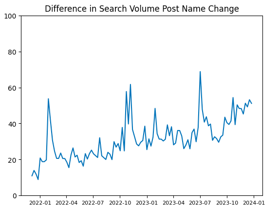
Summing these values over time, we get approximately +3300 search volume since the name change.

Based on the counterfactual, the expected search volume for the word ‘meta’ was ~2600 to EOY 2023. However, after the name change, search volume for ‘meta’ was actually about 6000. Therefore, there was an 130% increase in searches due to the name change.

Summary and Advanced Methods

In this article, I have shown how to do a simple Interrupted Time Series analysis, using search volume for the word ‘meta’ as an example. While straightforward, this method is particularly effective given that the appropriate assumptions are met.

I hope that you’ve found this article useful. If you wish to read more of my work, you can find the rest of my blog here. Alternatively, add me on Linkedin.

I’ve also made the code available on Github for reference.

Finally, there are a number of similar, more advanced methods that are beyond the scope of the article. These methods help to extend ITS beyond a single group or simple linear regression. I’ve provided some links below for reference.

ITS with ARIMA: extending ITS to non-linear time series
Bayesian Structural Time Series: advanced counterfactual creation
Bayesian Causal Inference: custom Bayesian implene
Hierarchical Multilevel Models: for measuring several groups or interventions at the same time

Aaron Pickering

Interrupted Time Series

Data

Assumptions

Confounding

Linearity

Target Distribution

Consistent Variance

Setup and Preprocessing

Interrupted Time Series Model

Code: Frequentist Approach

Code: Bayesian Approach

Model Diagnostics

Results

Counterfactual

Summary and Advanced Methods

Subscribe

Leave a comment Cancel reply

Interrupted Time Series

Data

Assumptions

Confounding

Linearity

Target Distribution

Consistent Variance

Setup and Preprocessing

Interrupted Time Series Model

Code: Frequentist Approach

Code: Bayesian Approach

Model Diagnostics

Results

Counterfactual

Summary and Advanced Methods

Subscribe

Share this:

Leave a comment Cancel reply