Bayesian Time Series Interpolation

To understand and make decisions about the world around us, we need to understand not only the most likely outcome but other less likely, but possible outcomes too. In the context of Data Science and Machine Learning that means going ‘Bayesian’, so to speak.

Previously, on my blog I discussed in detail a method for multivariate time series interpolation using linear basis functions. In the first article on the topic, I used a statistical approach; a Hierarchical Multilevel model which encodes the similarity between series with a group variable. In the second article, I went in the pure ML direction using categorical embeddings to learn relations between the series at scale using Pytorch. In today’s article, I will extend the hierarchical model approach making it fully Bayesian so that we can understand and explore the model’s uncertainty.

Conveniently, the model structure itself doesn’t change. We’ll use the same Hierarchical model and features as in the first article, while turning it Bayesian via the Numpyro and Bambi modelling frameworks.

On that note, let’s start with a quick recap of the problem setting. Alternatively, head directly to the model.

Data

First, lets simulate 100 random walks, each 100 time steps drawn from a multivariate Gaussian distribution with covariance = 0.6. This means that all the time series are related to each other and move in a similar direction per time step. However, they are also prone to drift apart over time.

# Set the number of time steps
n_steps = 100
# Set the number of random walks
n_walks = 100

# Generate random walks with the same mean and variance
np.random.seed(123)
cov_matrix = np.diag(np.zeros(n_walks) + 1)
cov_matrix[cov_matrix==0] = 0.6
random_walks = np.random.multivariate_normal(np.zeros(n_walks), cov_matrix, size=n_steps)
random_walks = np.cumsum(random_walks, axis=0)

Our task is to take one of the series, delete 95 of the 100 time steps and then try to reconstruct the series using Bayesian Time Series interpolation.

While we’ll look at a single series here, you can easily reconstruct any number of time series simultaneously.

Bayesian Hierarchical Model

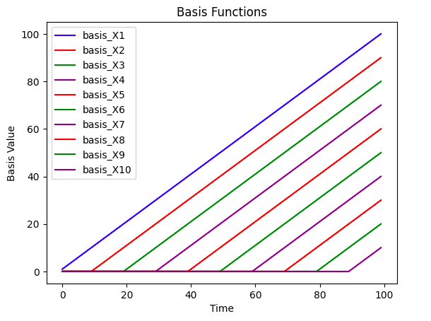
To effectively model the time series, we’ll create 10 linear basis functions that are equally distributed across time. The basis functions are plotted below below. Each individual time series will be modelled as a linear combination of the bases multiplied by their coefficients.

Note: Our model methodology has a key assumption i.e all of the series are correlated or related If the series aren’t related then this methodology will be ineffective, you’ll need to decide for yourself whether this assumption holds for your particular problem.

Model Formulation

Given basis functions $X_{1}$ through $X_{10}$ , our Bayesian model has the following formulation:

$y \sim \mathcal{N}(\mu, \sigma^2)$
$\large \mu = \beta_{1j} \cdot X_{1} + \beta_{2j} \cdot X_{2} + \beta_{3j} \cdot X_{3} + \beta_{4j} \cdot X_{4} + \beta_{5j} \cdot X_{5} + \beta_{6j} \cdot X_{6} + \beta_{7 j}\cdot X_{7} + \beta_{8j} \cdot X_{8} + \beta_{9j} \cdot X_{9} + \beta_{10j} \cdot X_{10} + \gamma_{j}$

with hierarchical terms for the $\beta$ values given by

$\beta_{nj} \sim \mathcal{N}(\beta_{n}, \theta_{n}^2)$

$\gamma_{j} \sim \mathcal{N}(\gamma, \zeta_{n}^2)$

with weakly informative priors:

$\beta_{n} \sim \mathcal{N}(0, 50)$

$\theta_{n} \sim \mathcal{N}^+(50)$

$\sigma \sim \mathcal{N}^+(10)$

$\gamma \sim \mathcal{N}(0, 5)$

Regarding the selection of priors, I have selected some generic, very weakly informative priors based on the variable ranges. This selection work fine but there are smarter ways to choose weakly informative priors, as discussed below.

Numpyro Code

To build the Bayesian model, I am using the probabilistic programming framework NumPyro. The code is shown below:

import numpyro
import numpyro.distributions as dist
from numpyro.infer import MCMC, NUTS
from jax import random

def bayesian_time_series_interpolation(X, y, level):
    # Prior distributions
    beta_1 = numpyro.sample("beta_1", dist.Normal(0, 50.0))
    theta_1 = numpyro.sample("theta_1", dist.HalfNormal(50.0))
    beta_2 = numpyro.sample("beta_2", dist.Normal(0, 50))
    theta_2 = numpyro.sample("theta_2", dist.HalfNormal(50))
    beta_3= numpyro.sample("beta_3", dist.Normal(0, 50))
    theta_3 = numpyro.sample("theta_3", dist.HalfNormal(50))
    beta_4 = numpyro.sample("beta_4", dist.Normal(0, 50))
    theta_4 = numpyro.sample("theta_4", dist.HalfNormal(50))
    beta_5 = numpyro.sample("beta_5", dist.Normal(0, 50))
    theta_5 = numpyro.sample("theta_5", dist.HalfNormal(50))
    beta_6= numpyro.sample("beta_6", dist.Normal(0, 50))
    theta_6 = numpyro.sample("theta_6", dist.HalfNormal(50))
    beta_7 = numpyro.sample("beta_7", dist.Normal(0, 50))
    theta_7 = numpyro.sample("theta_7", dist.HalfNormal(50))
    beta_8 = numpyro.sample("beta_8", dist.Normal(0, 50))
    theta_8 = numpyro.sample("theta_8", dist.HalfNormal(50))
    beta_9 = numpyro.sample("beta_9", dist.Normal(0, 50))
    theta_9 = numpyro.sample("theta_9", dist.HalfNormal(50))
    beta_10 = numpyro.sample("beta_10", dist.Normal(0, 50))
    theta_10 = numpyro.sample("theta_10", dist.HalfNormal(50))
    gamma_sigma = numpyro.sample("gamma_sigma", dist.HalfNormal(10.0))
    sigma = numpyro.sample("sigma", dist.HalfNormal(10.0))

    # Hierarchical term for each beta and level
    n_levels = 100
    with numpyro.plate("plate_i", n_levels):
        b1 = numpyro.sample("b1", dist.Normal(beta_1, theta_1))
        b2 = numpyro.sample("b2", dist.Normal(beta_2, theta_2))
        b3 = numpyro.sample("b3", dist.Normal(beta_3, theta_3))
        b4 = numpyro.sample("b4", dist.Normal(beta_4, theta_4))
        b5 = numpyro.sample("b5", dist.Normal(beta_5, theta_5))
        b6 = numpyro.sample("b6", dist.Normal(beta_6, theta_6))
        b7 = numpyro.sample("b7", dist.Normal(beta_7, theta_7))
        b8 = numpyro.sample("b8", dist.Normal(beta_8, theta_8))
        b9 = numpyro.sample("b9", dist.Normal(beta_9, theta_9))
        b10 = numpyro.sample("b10", dist.Normal(beta_10, theta_10))
        gamma = numpyro.sample("gamma", dist.Normal(0, gamma_sigma))

    # Calculate the mean
    mu = b1[level]*X[:,0]  + b2[level]*X[:,1] + b3[level]*X[:,2] \
    + b4[level]*X[:,3] + b5[level]*X[:,4] + b6[level]*X[:,5] \
    + b7[level]*X[:,6] + b8[level]*X[:,7] +b9[level]*X[:,8] \
    + b10[level]*X[:,9] + + gamma[level]
  
    # Likelihood
    numpyro.sample("obs", dist.Normal(mu, sigma), obs=y)

Model Training

Model training is easily done with the Numpyro MCMC samplers. In this case I will use the available NUTS sampler.

nuts_kernel = NUTS(bayesian_time_series_interpolation)
mcmc = MCMC(nuts_kernel, num_samples=3000, num_warmup=1000, num_chains=2)

# run the mcmc sampler
mcmc.run(rng_key=random.PRNGKey(0), X=X, y=y, level=level)

Simplified Formula Syntax with Bambi

Beyond the Numpyro syntax specified above, it’s also possible to use the simplified formula syntax of Bambi. Bambi is a Python package that acts as a wrapper for the probabilistic programming language PyMC.

In most cases, its a great option! Bambi does smart selection of noninformative priors behind the scenes, simplifying the model building process. Personally, I find the formula syntax much easier for many use cases.

model = bmb.Model("value ~ (basis_X1 | level) + (basis_X2 | level) + (basis_X3 | level) + (basis_X4 | level) + (basis_X5 | level) + \
(basis_X6 | level) + (basis_X7 | level) + (basis_X8 | level) + (basis_X9 | level) + (basis_X10 | level) + (1 | level)", sample_df, family="gaussian", categorical = "level")

Trace Plot & Diagnostics

After training the model, we can check some diagnostics to confirm convergence and see whether the model trained correctly.

MCMC Chains

Given the large number of parameters, I won’t visualize all of the available diagnostics.

Shown below are the chains for the first three basis $\sigma$ s. Importantly, they are roughly stationary and the posterior distributions are approximately normally distributed. Both chains produce similar results for each parameter indicating a high likelihood of convergence.

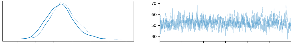
Finally, here is the chain for the first basis function $\beta$ . Notice on the left that there is one normal distribution per time series, while the collection of these distributions is also normally distributed. This is consistent with our hierarchical specification of the model.

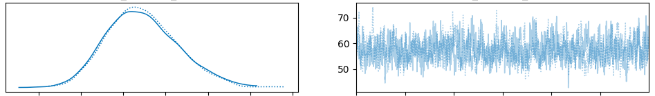
Fit Posterior

Below are some selected fits – the posterior predictive distributions for the first 3 time series.

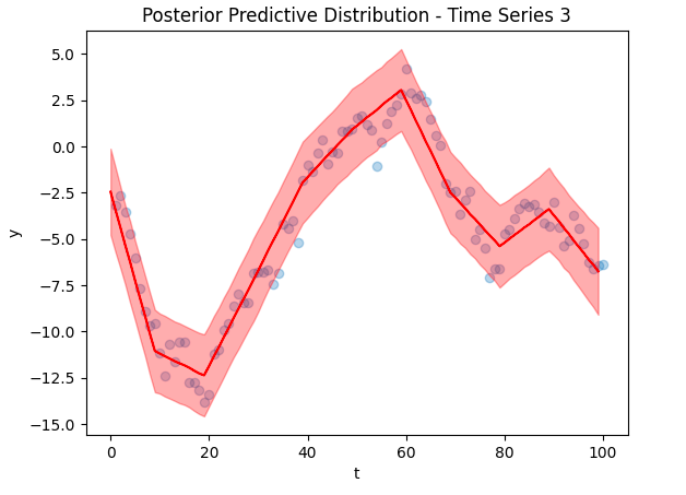
As you can see, the predictions fit the training data excellently, suggesting that our model was trained reasonably well. However, these plots are based on in-sample training data, we need to check the out of sample predictions for a truer picture.

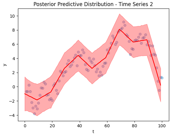
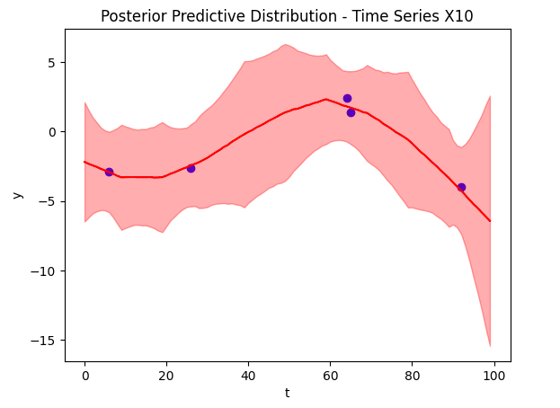
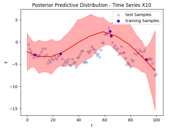
Posterior Predictions

Now to the crux of the article, our time series reconstruction! The figure below shows the reconstruction in red, with the deleted data points overlaid in blue. The posterior predictive distribution is the light red shaded region. Despite training on only 5 data points (and other time series), we were able to find an accurate reconstruction.

Conclusion

All in all, the Bayesian approach is an interesting addition to our multivariate time series interpolation model. By making some small changes we are able to generate posterior predictive distributions and have a better idea about our uncertainty.

In addition, writing the code and adapting the model is not particularly difficult given the availability of excellent modern tools such as Numpyro, PyMC and Bambi.

Aaron Pickering