Aaron Pickering

A common pattern I observe among inexperienced Data Scientists is the following: they often default to XGBoost or a similar Gradient Boosted Model for their problem without considering whether it’s the right choice for the job.

Given how powerful these methods are, this isn’t the most egregious mistake one can make. However, it’s important to understand the strengths and weaknesses of your models and tailor your choice to the needs of the problem. Let me give one example.

Despite being a machine learning powerhouse, XGBoost has a significant weakness: extrapolation. Extrapolation is the ability of a model to make predictions for data that falls outside the range of what it was trained on. This can be a serious problem when you’re working with time-series data or when your data-generating process changes over time. This is surprisingly common in real-world scenarios, as the world is constantly changing! This weakness in extrapolation is shared by all tree-based models that use constant functions between split points, e.g., Random Forest, XGBoost, LightGBM, etc.

But, don’t just trust me. Let me show you via an example.

The Example

Let’s start with a simulated dataset that highlights the problem. We’ll create a problem with a probabilistic target variable and 2 input features.

Here’s a quick look at how the data is set up:

• Target: Binary outcome (1 = success, 0 = failure)
• Price: A variable that drifts over time
• Day: Day number (1 to 50)

We split the data into a training set (first 20 days) and a test set (last 30 days).

import numpy as np
import pandas as pd
import matplotlib.pyplot as plt
import xgboost as xgb

num_days = 50
observations_per_day = 20
start_p = 0.9
end_p = 0.4

data = []
delta_p = (end_p - start_p) / (num_days - 1)

for day in range(num_days):
    # Simulate daily probability
    current_p = start_p + (day * delta_p)
    # Add some random daily component
    observations = np.random.binomial(1, current_p, observations_per_day)
    # Let's make the price based on past observations to simulate a drift
    price = current_p * 1000
    for obs in observations:
        data.append([day + 1, obs, price])

# Convert to a dataframe
df = pd.DataFrame(data, columns=['Day', 'Target', 'Price'])
df['Intercept'] = 1

Training a Model

We train an XGBoost classifier to predict the probability of success using the input features. After training the model, we’ll predict the probabilities for both the training and test sets and compare. Let’s see how the model does when extrapolating.

train_df = df[df['Day'] <= 20]
test_df = df[df['Day'] > 20]

# Features and labels
X_train = train_df.drop(columns=['Target', 'Price','Day'])
y_train = train_df['Target']
X_test = test_df.drop(columns=['Target', 'Price', 'Day'])
y_test = test_df['Target']

print(X_train.head())

# Train the XGBoost model
model = xgb.XGBClassifier(eval_metric='logloss')
model.fit(X_train, y_train)

# Predict probabilities for the training set
y_train_pred_proba = model.predict_proba(X_train)[:, 1]
train_df['Predicted_Prob'] = y_train_pred_proba

# Predict probabilities for the test set
y_test_pred_proba = model.predict_proba(X_test)[:, 1]
test_df['Predicted_Prob'] = y_test_pred_proba

# Calculate the mean of the target variable and predicted probabilities for each day in both sets
daily_means_train = train_df.groupby('Day')['Target'].mean()
daily_probs_train = train_df.groupby('Day')['Predicted_Prob'].mean()
daily_means_test = test_df.groupby('Day')['Target'].mean()
daily_probs_test = test_df.groupby('Day')['Predicted_Prob'].mean()

Extrapolation Issue

XGBoost excels at fitting data within the range it saw during training, but struggles when predicting for values outside this range. In our case, the model is trained on the first 20 days, and when tested on days 21-30, the predicted probabilities don’t follow the actual trend.

We can visualize this by comparing the predicted probabilities against the actual target values over time. The plot below reveals that the model fits the training data well but starts to diverge when it reaches the test data.

# Plot the mean target variable and predicted probabilities per day
plt.figure(figsize=(10, 6))
plt.plot(daily_means_train.index, daily_means_train.values, marker='o', linestyle='-', color='blue', label='Mean Target (Train)')
plt.plot(daily_probs_train.index, daily_probs_train.values, marker='x', linestyle='--', color='green', label='Mean Predicted Probability (Train)')
plt.plot(daily_means_test.index, daily_means_test.values, marker='o', linestyle='-', color='orange', label='Mean Target (Test)')
plt.plot(daily_probs_test.index, daily_probs_test.values, marker='x', linestyle='--', color='red', label='Mean Predicted Probability (Test)')
plt.title('Mean of Target Variable Per Day and Predicted Probabilities')
plt.xlabel('Day')
plt.ylabel('Mean Target / Predicted Probability')
plt.legend()
plt.grid(True)
plt.show()

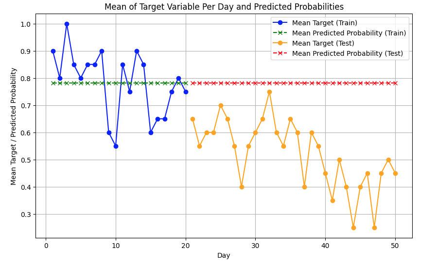
Notice how the prediction also remains flat outside of the training range? In many applications that type of extrapolation property would be completely unreasonable. So clearly, it struggles with trends.

Let’s try another example, even simpler. We’ll just check if XGboost can predict an obvious value outside of its training range. To do that, I’ve simulated a simple line y = 2x, plus a little bit of noise.

np.random.seed(0)

# Simulate data y = 2*x + noise
def true_fn(x):
    return 2 * x + np.random.normal(0, 0.5, size=x.shape)

# Train only on x in [0, 10]
x_train = np.linspace(0, 10, 200).reshape(-1, 1)
y_train = true_fn(x_train.ravel())

# Predict on extended range (includes outside [0, 10])
x_full = np.linspace(-5, 15, 300).reshape(-1, 1)
y_true = 2 * x_full.ravel()

model = XGBRegressor(n_estimators=50, max_depth=3, random_state=111)
model.fit(x_train, y_train)
y_pred = model.predict(x_full)

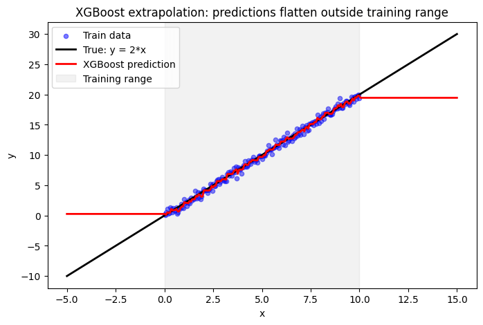
Completely flat prediction outside of the training range.

Why XGBoost Struggles with Extrapolation

XGBoost builds a series of decision trees based on the training data and creates rules that split the feature space. By default, these splits are constant, and outside the training range, the constants are simply extended outwards. So, if your training data is non-stationary, constant extrapolation will fail.

As you can imagine, there are many scenarios where this is not appropriate. In fact, many of your problems may suffer from this to some degree. Often, time-based trends and market dynamics are present in machine learning problems, so be sure to watch out for this trap!

What Can you Do Instead?

There are a variety of ways to mitigate this issue. Many people simply retrain the model regularly, ensuring that the latest data is always in the training set and the model doesn’t have to extrapolate very far. For time-series problems, practitioners often add carefully constructed feature sets, such as lags, rolling windows, and other time components. You can also try target transformations, including differencing or scaling.

Finally, choose a model whose properties match your problem! Gradient boosting models are the default these days, but you don’t need to use them for every problem.