Aaron Pickering

Some weeks back in part 1, I introduced the concept of heteroscedasticity and demonstrated the importance of dealing with it when doing analysis and modelling.

In it I tackled heteroscedasticity through variable transformations and simple linear regression models. However, life is not always so straightforward. I also promised to show techniques for handling more complicated heteroscedastic problems – and that’s exactly what I’ll do!

In this post, I’ll look at dealing with heteroscedasticity in inference problems. Specifically, I’ll illustrate how to handle problems with challenging elements such as:

• Strong trends
• Non-linearity
• Non-normal target distributions
• Multiple seasonalities
• And above all, changing variance

While I’ve added some code here and there in this article, you can find the complete, reproducible notebook via my Github page. Let’s get into it.

Simulated Data

For this post, I created a simulated data set and problem but chances are high that you may have seen something similar in your own work.

For businesses, products or metrics that are growing, there will often be a strong upward trend. And when growth occurs, the variance tends to grow with it e.g more sales leads to more variation in sales. This type of heteroscedastic problem is all too common and rarely addressed – that’s why I have chosen it for our simulated example.

For the problem I generated a time series called “Sales” which grows over time. The time series appears to have some seasonal patterns, so we’ll have to look into that. And the variation is clearly getting bigger over time – that’s the heteroscedastic component. You can see the time series in the image below.

Finally, I have added a simulated ‘marketing spend’ response. For this exercise, we’d like to retrieve the relationship between marketing spend and sales as accurately as possible. The actual value of the beta is 1, let’s see if we can capture that later.

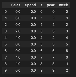
For reference, the dataset itself has the following structure (first 10 rows):

Again, just a reminder that this in an inference problem not a forecasting problem and that the model has been chosen accordingly.

How can we model such a time series to understand the underlying dynamics and relationships between the variables?

Bayesian Spline Models

One possible option is to use a Bayesian Spline Model with Conditional Variance. The naming here is complicated but breaking it down we have three important terms:

• Bayesian: a modelling technique that let’s us understand the probability distributions and uncertainty behind our problem
• Spline: Spline models are simply a combination of curves (polynomials) that can be used to model complex non-linear functions. Spline functions have the benefit of being flexible, powerful and importantly, explainable.
• Conditional Variance: In a traditional regression model, we’d try to predict only the mean or the ‘best fit’. However, in a conditional variance model we try to model the uncertainty as well. If you need a refresher, refer to part 1 for details.

From a practical implementation perspective, PyMC is the perfect choice for this problem. With PyMC you can build Bayesian models of nearly any complexity and it has a fantastic ecosystem surrounding it. I highly recommend it.

Next we have to specify our spline regression parameterisation. To do this, you’ll need to think about the components needed in your model. For time series, of the most common ways is to use a decomposition technique. Typically, the time series is decomposed into trend, seasonal and remainder components. Each of these components can be significantly complex in their own right. The decomposition process helps to explicitly capture and model trends which can violate typical regression stationarity assumptions, and seasonalities which are the most common explanatory factors in time series.

Back to the three components. The trend is a slow moving curve that represents general growth or decline. The seasonal component models repeating patterns. The remainder component is just the leftovers- typically external regressors (e.g marketing spend) and noise.

In addition, we need to make sure that we are using the right model family. To do that we need to check the distribution of the sales variable. We need to be a bit careful about this because the trend distorts the actual distribution. If we look closely at the first 50 time points (left), we can see that the values are bounded at 0 and they are definitely skewed. We can also see this represented via a histogram (right)

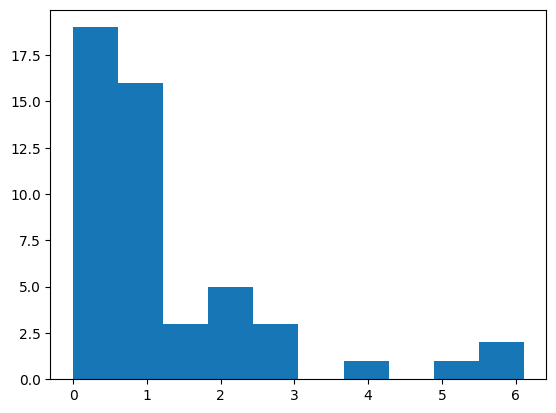
Given this, we need to pick an appropriate target distribution. The negative binomial distribution is a common choice for this type of data.

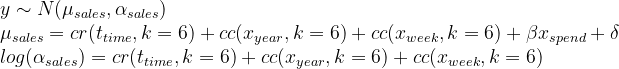
Putting all together, we’ll use the Negative Binomial model family and we need to model both the mean and the dispersion. We also need to model the seasonality in each.

Finally, we need to add the marketing spend. I’ve chosen a linear term but you could use whatever complexity you feel is required. The overall equations for our model are shown below.

Spline Equation

The associated python code can be found via my Github page.

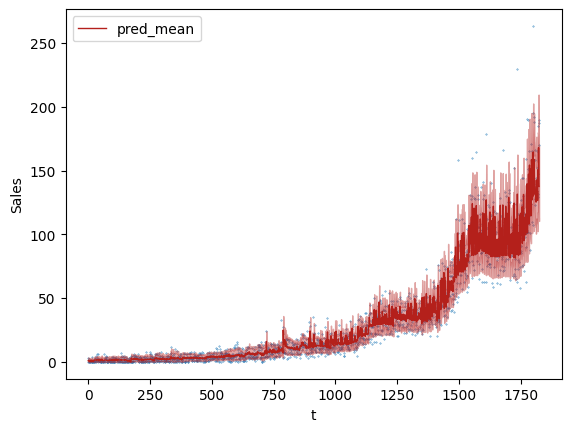
After running the code and completing the inference, we get the fit shown below. Looks pretty good! The dark red line captures the predicted mean, and the lighter shade captures the uncertainty (~95%). You can see that the uncertainty changes and grows, indicating that we have correctly captured the heteroscedasticity.

If you want, you can also check the calibration; approximately 5% of the blue points fall outside of the band as expected.

We can also extract the estimated relation between spend and sales. The estimated beta value is 0.09 as shown in the table below. That’s very close to the actual value of 1!

Bayesian Additive Regression Trees

Just before I wrap up the post I’d also like to highlight an alternative option for the modelling – Bayesian Additive Regression Trees. Without going into any detail, they are basically the Bayesian variant of the Random Forest. BART models have many of the same benefits as the spline models for inference. In my experience, they are a little slower to train and marginally less interpretable, but are easier to set up and require less experience to handle. They are a great choice!

For more information, the PYMC docs have a good introduction,
and a more comprehensive example, for cohort and revenue retention, can be found here.

Back to the modelling, the formula specification for a BART model is much simpler. You don’t need to explicitly add seasonality or the marketing spend, that’s all covered by the generic function (f). The model takes care of learning all the important features.

In doing so, you leave yourself to the model somewhat. Be aware that you may need to have the right input variables and feature engineering for this to work properly.

BART Model Equation

Full code can can be found here.

Finally, plotting the fit, we get the image below. You can see that it properly captures both the mean and the dispersion, with very similar results to the spline model. If you have a good eye, you might notice that the prediction interval is more ‘spiky’ than the spline model. That’s because the uses multiple decision trees rather than polynomials for constructing the relevant functional relationships.

However, all in all the BART model works very well.

Summary

Strongly heteroscedastic problems can be very tough. Add trends, non-linearity and non-normal target distributions and they get even more challenging. However, there are options.

In this blog post, I’ve shown how you can work with heteroscedastic data both a Bayesian Spline model and a BART model. As you can see, both are effective and powerful tools. Try them out next time you run into a heteroscedastic problem!

Finally, you might have noticed that, so far, I have not touched on the topic of forecasting at all. In my next article, I’ll finish my series on heteroscedasticity and tackle a complicated, non-linear time series forecasting problem with Pytorch.

---

Subscribe