
How can you run a Bayesian A/B tests with PyMC?
What if you have multiple choices e.g A/B/C test or a multivariate test?
This blog post shows how you do this kind of test using PyMC, in a fully Bayesian way. Why use Bayesian methods? Personally, I prefer to think in terms of probabilities and to fully understand the uncertainty present in the problem. Bayesian methods provide a nice framework for this type of thinking. Overall, this is a fairly simple procedure so I thought I’d note it down for posterity, feel free to copy it for your experiments.
Simulated Data
Lets get started with some sample data. Lets say we conduct a trial of our product with three equal groups (A,B,C) and we which to see which ones has the best conversion rate. For each trial we note a conversion as 1 or 0 otherwise.
def create_sample(trials_a,
                  conversions_a,
                  trials_b,
                  conversions_b,
                  trials_c,
                  conversions_c):
  ''' Function that generates data for three groups A, B, C with n trials and n conversions '''

    outcome_a = np.zeros(trials_a)
    outcome_a[:conversions_a] = 1
    outcome_b = np.zeros(trials_b)
    outcome_b[:conversions_b] = 1
    outcome_c = np.zeros(trials_c)
    outcome_c[:conversions_c] = 1

    level_a = pd.DataFrame({"group":np.repeat("a", trials_a), "outcome":outcome_a})
    level_b = pd.DataFrame({"group":np.repeat("b", trials_b), "outcome":outcome_b})
    level_c = pd.DataFrame({"group":np.repeat("c", trials_c), "outcome":outcome_c})

    df = pd.concat([level_a, level_b, level_c], axis=0)
    cats = pd.get_dummies(df['group'])
    df = pd.concat([df, cats], axis=1)
    df = df.drop("group", axis=1)

    return df
Our data looks like this
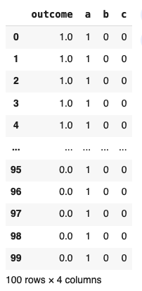
with the respective number of trials and conversions provided below:
| Group | # Trials | # Conversions |
| A | 100 | 50 |
| B | 22 | 14 |
| C | 1000 | 650 |
Bernoulli Model
Many people will choose to do the calculations using the aggregated numbers and the Binomial distribution, which works well. I prefer to keep the trials distinct and treat it as a regression model of the Bernoulli family. This is just a personal preference, I find interpretation and customization easier.
A Bernoulli distribution can be either 0 or 1 with probability p.
Logistic Link Function
To model the Bernoulli distribution, we perform a linear regression with a logistic link function (similar to a classification model in the machine learning parlance).
Modelling Code – Pymc & Bambi
Thankfully, using the package Bambi, the difficulties in the setup are taken care of for us. Bambi is a wrapper around PyMC which allows us to directly specify the model with formula objects. Its really straightforward to use. We just need to specify a family parameter – in this case Bernoulli.
model = bmb.Model("outcome ~ a + b + c - 1", df, family="bernoulli")
results = model.fit(draws=10000, chains=10)
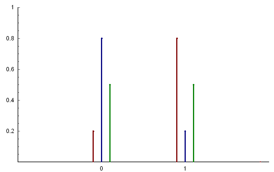
az.plot_trace(results, compact=False)

The images above left show the estimated distributions for each group parameters for A, B & C.
The values themselves are not the proportions ‘p’ yet, you’d need to pass them through a logistic function to get that value. However, from the distributions we can easily see which group was better.
Outcome
Just eyeballing things, we can clearly see that group A is the worst of all. Its average value is around zero, much lower than the other two. We can simply rule that group out of contention.
Regarding the other groups, lets look at the estimated values:
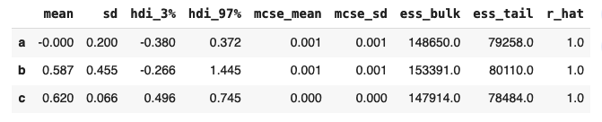
Group C has the highest mean value and importantly, the standard deviation is quite narrow indicating high certainty.
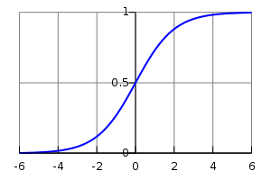
To get the actual estimate, we need to pass the values through a logistic function. The logistic function is given by:
def logistic(x):
  return 1/(1 + np.exp(-x))
And taking logistic(x) where x is the mean value of 0.62, we get a conversion rate of 0.65 – exactly equal to our simulated conversion rate.
One more question though, the mean for group B is actually pretty close to the mean for group C. How certain are we that B is actually worse?
To answer that, lets check the posterior chains (generated during fitting) and see with what probability B was less than A.
comparison = np.ndarray.flatten(np.array((results.posterior['c'] > results.posterior['b'])))
np.sum(comparison)/len(comparison)
This code essentially counts how often C was greater than B is the posterior draws of the modelling process and divides by the total number of draws. Since the posteriors define the conversion rate distributions of the two groups, the resluting value gives us the probability that C is greater than B.
From this we calculate that C is greater than B with 54% probability. So, the result is actually quite close.
In fact, the confidence interval of the parameter p for group B ranges from approximately 0.25 to 0.9. If you like to live dangerously, perhaps B is the right choice! But more seriously, C is likely the best outcome here, supported by the given distributions and numbers.

Leave a reply to How to Choose a Distribution for your Regression Model – Aaron Pickering Cancel reply