Aaron Pickering

In most resources on time series data, its a given that the time series are complete i.e there is a consistent one measurement per time interval.

However, in a lot of applications this isn’t the case. Sometimes the data is there are a just few holes here and there. There are a lot of techniques for this type of missingness. But what if the time series is sparse?

What if you are missing 95%+ data points per series or only have a small handful of data points to draw from? How can you handle this type of data?

One way is to leverage information from other similar time series. If your time series sit in a hierarchy e.g one series per country, city, person, group etc, then you may be in luck.

This is particularly true if you suspect the time series are derived from the same process, differing a little between the groups.

In this post I will interpolate a time series with less than 10 data points by drawing information from other, similar time series.

Simulated Example

For those of you that follow my blog, you’ll know that for educational purposes I like to work with simulated data because you can assess precisely the accuracy of your solution. This post is no different.

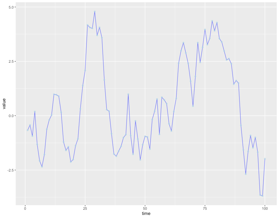
For this example, I have generated 100 time series. The time series themselves are 100 step random walks drawn from a multivariate Gaussian distribution with covariance = 0.6. This means that all the time series are related to each other and move in a similar manner over time. However, they move in differently on a local level and are prone to drifting over time.

Here are the time series:

The series are similar but wax and wane over time as small differences add up.

Goal

For this exercise, we’re going to take one of these time series, delete 97 data points and then try to reconstruct it without looking.

Here’s the full series:

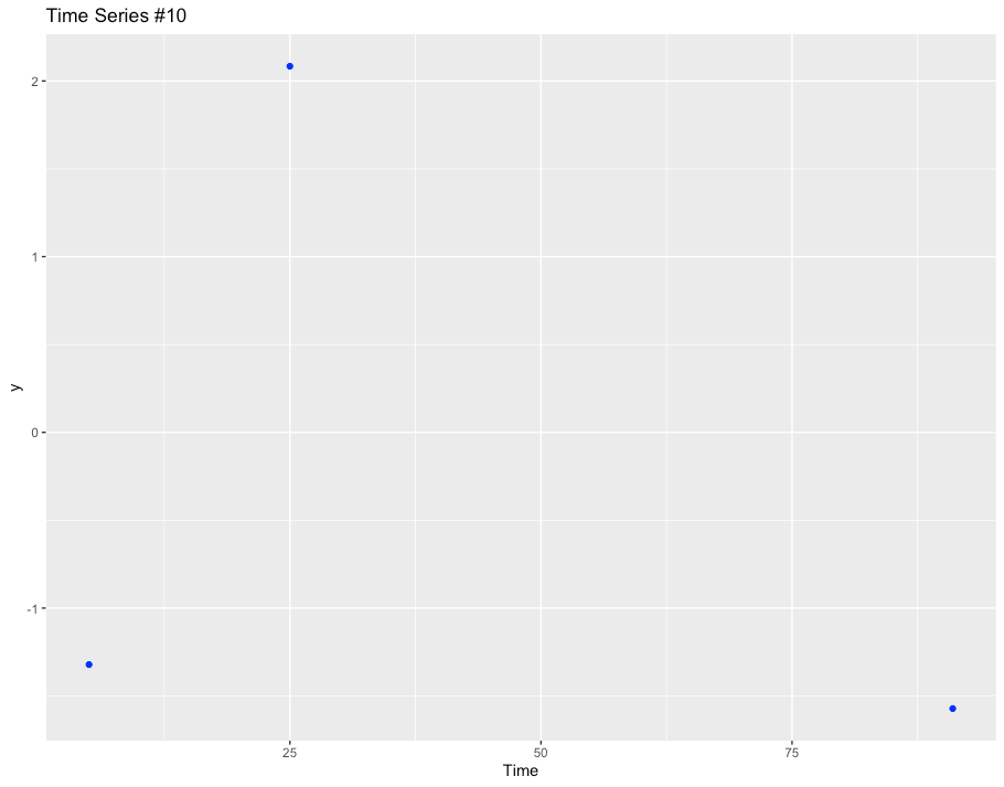
And below is the time series we will reconstruct from. Not a lot of data to work with!

The Model

How can we possibly reconstruct the time series accurately given just three points!?

If we build our model based on this series alone we’ll go nowhere. To get a good result we’ll need to leverage information from the other 99 time series. But how?

We need to account for two critical aspects:

1. Our model should learn the relationship between the time series to support information sharing.
2. Our model should learn the movements over time of each series.

Note:
The following model is a trend only model and is not reflective of the data generating process itself. Given that these are random walks, this model is suitable for interpolation but not forecasting.

Learning the Relationships between Time Series

To do this, we’ll use a Hierarchical Model (also called Mixed Effects or Random Effect). I discuss Hierarchical Modelling in more detail in this article but essentially Hierarchical modeling (also known as mixed-effects modeling or multilevel regression) is a statistical technique used to analyze data that has various levels. In our case, we’ll treat each time series as its own level.

In a Mixed Effects model the parameters (betas, slopes, whatever) each vary a little by level. So the entire dataset has an average parameter (or fixed effect), which is a little higher or lower for each time series.

Each parameter shouldn’t be too far away from the others, and the “force” which keeps them close is a shared parameter mean and standard deviation (assuming a Gaussian relation) in the likelihood (loss function).

Learning the movement over time of each series

However, learning the relationships between the series is useless if we can’t model the movement of each individual series over time.

To do that we’ll need to choose a time series model. There are many, many different time series models with various properties and, probably, quite a few of them would be suitable here.

However, I’d like my model to have the following properties:

• Simple model with few parameters
• Suitable for non-stationary trend components
• Powerful enough to learn strongly non-linear functions
• For ease of fitting, avoids recurrent learning structures e.g RNN, ARIMA, ETS

Therefore, I’ve decided to model the time series as combinations of linear basis functions.

A basis is a function that, when combined with appropriate coefficients, can approximate or represent a wide range of other functions or data patterns.

Simply, the target is represented by the sum of a bunch of functions, each scaled by a coefficient.

For example, if you have basis functions x₁, x₂, x₃ etc and coefficients a₁, a₂, a₃, your model becomes

y(t) = a₁x1(t) + a2x2(t) + a₃x3(t) + ...

For this problem, I have split the time domain into 10 basis functions. Each basis function is linear above t=k and 0 below. Side note: you might notice that they look like RELU activation functions). The basis functions are shown in the image below:

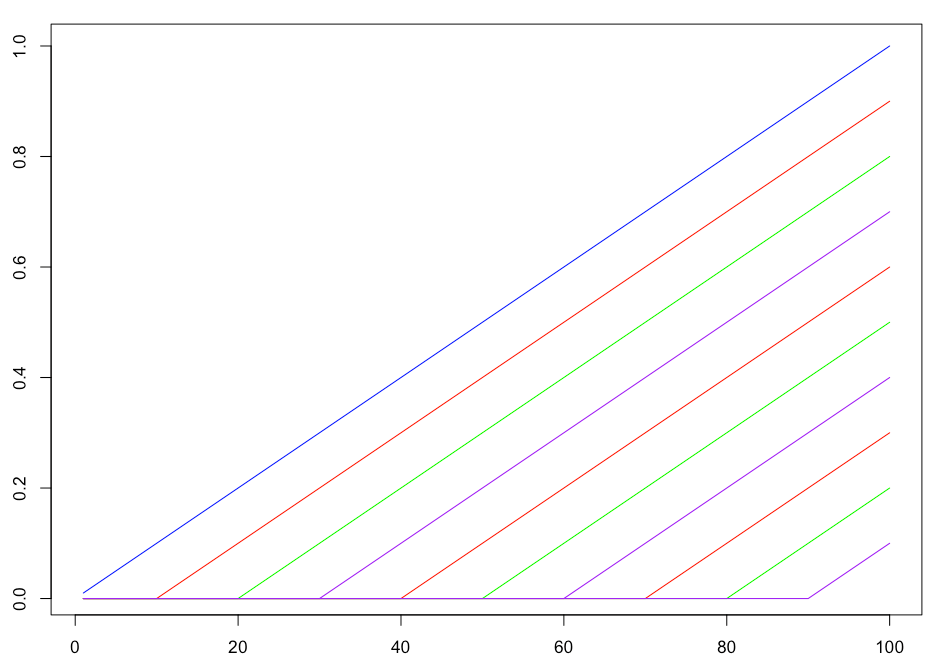
So, we multiply each basis by a slope and then sum them together. Don’t forget that we do this for each time series simultaneously, and the basis slopes between the time series are related by the Gaussian distribution.

That’s really the trick here, each time series has its own slope per time period, but crucially, that slope should be similar to the slopes of the other time series.

While the use of basis functions might sound very complex, its actually a fairly straightforward technique to implement. Essentially our time series model is 10 lines glued together. You’ll see that in the examples further along.

In fact, there is a very popular time series model that uses a very similar structure for its trend component – the Prophet model by Facebook.

Combining the two parts

Now we need to build the model.

There are many packages for building Hierarchical (Mixed Effects / Random Effects) models. For its user friendliness and easily readable formula syntax, I have chosen to use the lme4 package from R for the example below.

However, I’ve also written the same functionality in Python’s statsmodels and Pytorch. Relevant Python code can be found in my Github repo and the Pytorch model is also shown at the bottom of this article.

Continuin on, to fit the code using lme4 in R we use the following code:

f = as.formula("y ~ (1 | level) + (basis_X1 - 1 | level) + basis_X1 + (basis_X2 - 
    1 | level) + basis_X2 + (basis_X3 - 1 | level) + basis_X3 + 
    (basis_X4 - 1 | level) + basis_X4 + (basis_X5 - 1 | level) + 
    basis_X5 + (basis_X6 - 1 | level) + basis_X6 + (basis_X7 - 
    1 | level) + basis_X7 + (basis_X8 - 1 | level) + basis_X8 + 
    (basis_X9 - 1 | level) + basis_X9 + (basis_X10 - 1 | level) + 
    basis_X10")

lm_fit = lmer(f, data=sample_df)

Running this code, we simultaneously fit 100 time series models, each constructed from 10 linear basis functions. In addition, the coefficients for each time series are related by a Gaussian likelihood.

Results

Lets have a look at the results!

To be successful, our model should fulfill two criteria. Firstly it should provide a good fit for each of the 99 complete time series. Secondly, it should be able to use that information to make a decent reconstruction of Time Series #10 and its 3 remaining data points.

So lets start with the first criteria and look at some of the time series fits. Here are the first three time series in the set.

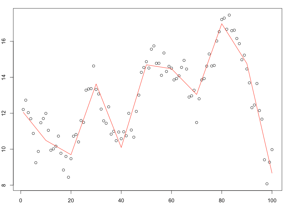
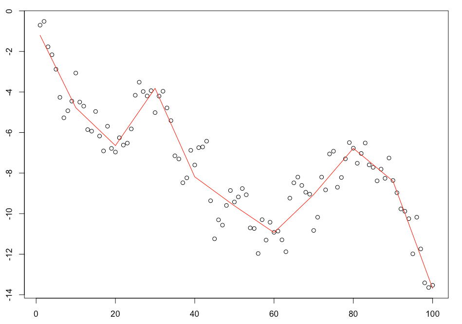
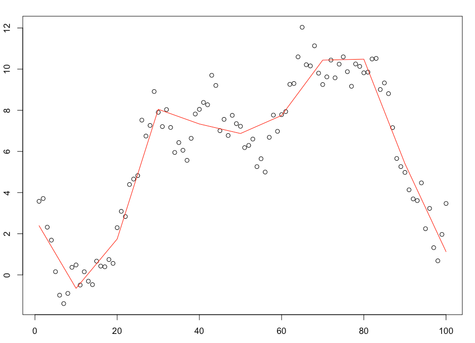
The fits look reasonable and the trends follow the time series closely. Its also worth noting that we can make the trend fit the data points further by increasing the number of basis functions used. I used 10 but you could easily increase that number and tighten the fit further.

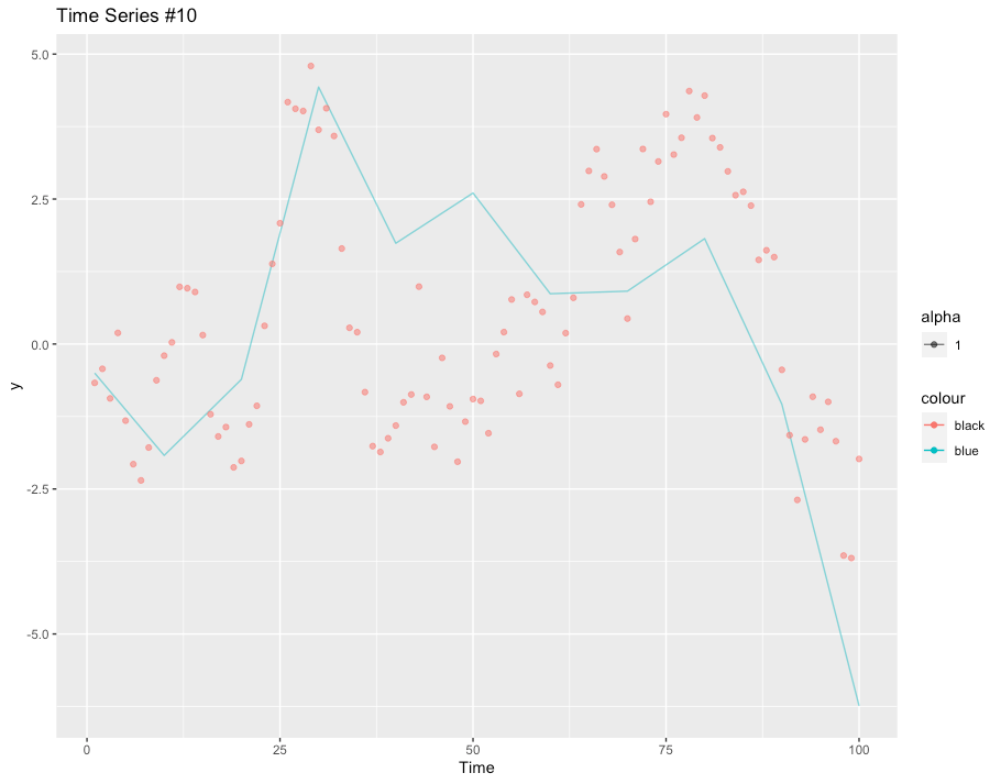
Now for the important part, lets look at our reconstruction. The image below shows the actual time series (red) with the reconstruction in blue. Its not bad, considering we only had the three points! It doesn’t capture every trend, but its much better than a naive guess.

Remember, we were reconstructing the series from this:

What were to happen if we were to retrain the model, instead interpolating between 6 data points rather than 3? You can see the results in the image below, a near perfect fit!

As you can see, this technique can be quite effective in the right conditions. Of course, you need multiple correlated time series and in practice that’s not always possible. But given that, this technique could be the right choice for your problem.

Feel free to try it for yourself!

Subscribe

Pytorch Model

As mentioned, I also built the same model with Pytorch and the code is shown below for reference. The complete notebook is also available via my Github. Finally, this approach treats each time series as a completely individual category and there are scaling limits with this approach. A nice extension would be to change the categories to an embedding layer. Next time!

class MixedEffectNetwork(nn.Module):
    def __init__(self, n_level, n_basis):
        super().__init__()

        self.n_basis = n_basis
        self.n_level = n_level
        # Linear Layers
        self.F = nn.Parameter(torch.rand(n_basis))

        # Overall intercept
        self.intercept = nn.Parameter(torch.rand(1))

        # Intercept random effect
        self.R_int = nn.Parameter(torch.rand(n_level))

        # Basis slope random effects
        self.R_effect = nn.Parameter(torch.rand(n_level, n_basis))

        # Additional parameter layers
        self.sd1 = nn.Parameter(torch.tensor(1.0)) # Error

        # Random effect regularisation
        self.u2 = nn.Parameter(torch.ones(n_level, n_basis))
        self.sd2 = nn.Parameter(torch.ones(n_level, n_basis))

        # Intercept random effect regularisation
        self.u3 = nn.Parameter(torch.ones(n_level))
        self.sd3 = nn.Parameter(torch.ones(n_level))


    def forward(self, X, L):

        # Fixed effects
        xf = torch.matmul(X, self.F)

        # Random effect intercept
        lr = torch.matmul(L, self.R_int.unsqueeze(1))

        # Random effect slopes
        lr_slope = torch.matmul(L, self.R_effect)
        X = X[:,:,None]
        lr_slope = lr_slope[:, None, :]
        lrx = torch.matmul(lr_slope, X)

        # Sum them all together
        y_p = lrx.squeeze(1).squeeze(1) + self.intercept + lr.squeeze(1)  + xf

        return y_p

    def loss(self, y_p, y):

        # Get the log likelihood for each of the random effect parameters
        l2 = 0
        for i in range(self.n_level):
          for j in range(self.n_basis):
            l2_dist = dist.Normal(self.u2[i,j], torch.exp(self.sd2[i,j]))
            l2 =+ l2_dist.log_prob(self.R_effect[i,j] - self.u2[i,j])

        l3 = 0
        for i in range(self.n_level):
          l3_dist = dist.Normal(self.u3[i], torch.exp(self.sd3[i]))
          l3 =+ l3_dist.log_prob(self.R_int[i] - self.u3[i])

        # Get the log likelihood for the error
        l1_dist = dist.Normal(0, torch.exp(self.sd1))
        l1 = l1_dist.log_prob(y - y_p).sum()

        # Sum them together and then scale them via the mean
        l = (l1 + l2 + l3) / ((self.u2.shape[0]*self.u2.shape[1]) + y.shape[0] + self.u3.shape[0])

        return -l