Aaron Pickering

In the 2001 article ‘Statistical Modeling: The Two Cultures’ Leo Breiman, famous for his work on Classification and Regression Trees, talks of two cultures of modelling. Loosely, the data modelling (statistical) and the algorithmic approaches.

In my previous article, I explored a method for Time Series interpolation using Mixed Effects (also called Random Effects or Hierarchical) models. In it, I interpolated and reconstructed a time series from only 3 points by drawing information from it’s multivariate neighbours. That was the statistical modelling school.

If you want to catch up on the background, you can check it out here.

This time, I’ll draw from the algorithmic school to solve the same problem using Pytorch and categorical embeddings. Finally, I’ll take you through some of the pros and cons of both approaches.

But first, a quick recap…

Recap

Skip the recap and head straight to the embedding model

My previous article, addressed the challenge of filling missing values in time series data, particularly when dealing with sparse datasets.

The solution involved drawing information from other similar time series to fill the missing data. We can do this if the time series share a hierarchical structure, such as one series per country, city, or group.

The example I gave was a simulated example with 100 related time series generated from a multivariate Gaussian distribution. For one of the series, most of the data points were removed and then through a model, reconstructed.

The model itself was a Mixed Effects model with linear basis functions to capture the relationships between time series and their movements over time. The mixed effect model incorporated a shared parameter mean and standard deviation on the coefficients to ensure that individual time series parameters were related to each other. The linear basis functions were used to represent the trend components of the time series, allowing for interpolation.

The reconstruction is shown in the image below.

Categorical Embeddings

Alternatively, what would be a Machine Learning solution to this problem? The trick is to use categorical embeddings.

In many machine learning tasks, categorical variables are one-hot encoded, where each category is represented by a binary (0 or 1) indicator variable. However, this leads to high-dimensional and sparse input representations as the number of categories increases. In the end, it becomes difficult for your model to learn anything of relevance.

Categorical embeddings map each category to a continuous vector space, normally with much lower dimensionality.

To give an example, consider that you have N=100 different time series. We might decide to one-hot encode this with N-1 = 99 new binary features. However, if we use an embedding, we feed our model with a single vector containing numbers 1 to 100 that map to our unique time series. Then, the embedding layer learns a numeric representation, converting each number to vector.

We can set the size of the embedding to whatever value we choose. The smaller the number, the more compression we have. An example of an embedding with size 3 is shown below.

Most famously, categorical embeddings are used in the field of Natural Language Processing, where each word is converted to a unique embedding rather than one-hot encoding the whole vocabulary of a language.

Why use Embeddings?

Embeddings are a good alternative to the Mixed Effects method for a number of reasons.

Firstly, scaling. Its easy to handle 100 one-hot encoded features but 1000, 10000, 100000? Soon, the size of your training data will explode with sparse features. An embedding provides dimensionality reduction allowing for scaling.

Next, the process of compressing the data into a smaller space forces the model to learn new representations of the data. These representations help to find similar time series – information which can be used for interpolation.

Finally, by using an embedding layer within a neural network we have the flexibility to model other dependencies and create customization. For example, we could include another layer that uses additional variables to model short term movements and interactions. This would be much harder to achieve with a linear Mixed Effects model.

Why wouldn’t you use Embeddings?

Well, for better or worse, using a Mixed Effects model we can encode our assumptions much more rigidly. Its easier to ensure our model conforms to and learns certain properties. In contrast, the embedding layer learns whatever provides the best fit, which is often but not always what is required for the problem.

Also, embeddings are generally less interpretable. Its harder to visualise a multidimensional embedding in comparison to straightforward regression coefficients. On the same note, the embeddings are not easily decomposable. The Mixed Effects model has trend, fixed effects and random effects which are easy to separate and understand.

The Model

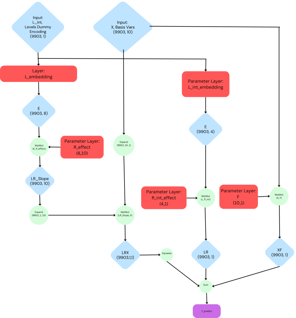
All that said, here is the construction of our final model. It contains the following components:

• Two data inputs: a numeric variable which uniquely represents each time series and a matrix of linear basis variables
• Embedding layers for the slopes and intercepts with dimensions 8 and 4, respectively.
• Three parameter layers which help to model the intercept, average effect and time series specific effects. While these could be combined, having three separate layers helps the model to learn global and local properties necessary for interpolation.

A complete visualisation of the network can be seen in the diagram below and notebook with code can be found on my Github page.

Visualising the Network

Results & Conclusion

Finally, the result of our reconstruction is shown below. Not bad at all!

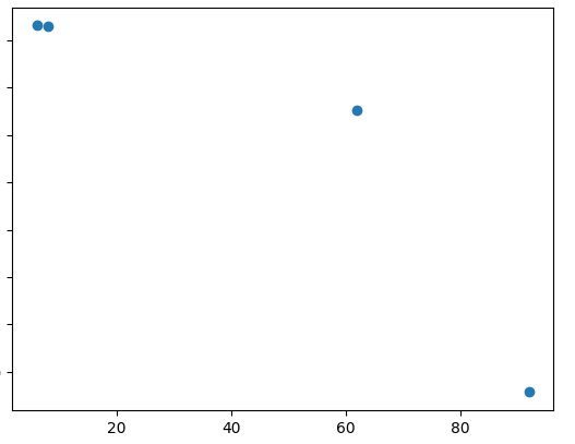
As you can see, this type of network with linear basis functions and embeddings could be a good choice for interpolating multivariate time series. Compared to the Mixed Effects (Hierarchical) approach, its a little more cumbersome but with has advantage of better scaling and the ability to customise and solve downstream tasks.

What I would like to emphasize is that the statistical and machine learning approaches have many parallels. In my opinion, its best to learn from the similarities and differences and always choose the best tool for the job at hand. Don’t be dogmatic.

Once more, complete code for this approach and the statistical approach can be found on my Github page. Alternatively, the Pytorch module is shown below.

Subscribe Below

Pytorch Code

class EmbeddingTrendNetwork(nn.Module):
    def __init__(self, n_level, n_basis, embedding_size):
        super().__init__()

        self.n_basis = n_basis
        self.n_level = n_level

        # Fixed effect parameters
        self.F = nn.Parameter(torch.rand(n_basis))

        # Intercept
        self.R_int = nn.Parameter(torch.rand(embedding_size, 1))

        # Slope parameters
        self.R_effect = nn.Parameter(torch.rand(embedding_size, n_basis))

        # Embedding layer for slopes and intercepts
        self.L_embedding = nn.Embedding(n_level+1, embedding_size)
        self.intercept_embedding = nn.Embedding(n_level+1, embedding_size)

        # Error std parameter
        self.sd1 = nn.Parameter(torch.tensor(1.0)) # Error sd


    def forward(self, X, L_int):

        # Fixed effect
        xf = torch.matmul(X, self.F)

        # Embedding for the intercept
        E = self.L_embedding(L_int)
        L_intercept = self.intercept_embedding(L_int)

        intercept = torch.matmul(L_intercept, self.R_int)

        # Embedding for the slopes (similar to the random effect)
        lr_slope = torch.matmul(E, self.R_effect)
        X = X[:,:,None]
        lr_slope = lr_slope[:, None, :]
        lrx = torch.matmul(lr_slope, X)

        # Sum the components
        y_p = lrx.squeeze(1).squeeze(1) + intercept.squeeze(1) + xf

        return y_p

    def loss(self, y_p, y):

        # Get the log likelihood for the error
        l1_dist = dist.Normal(0, torch.exp(self.sd1))
        l = l1_dist.log_prob(y - y_p).mean()

        return -l