Mutual Information

Many of us rely on Pearson Correlation as part of the exploratory data analysis process, to identify relationships between feature inputs and the target variable. In general, it’s a great option. However, in case you haven’t heard of it – next time consider trying Mutual Information (MI) as well. MI allows you to also discover non-linear relationships between variables, which makes it a powerful addition to your toolset.

What is Mutual Information (MI) ?

Mutual information is a measure of the amount of information that one random variable contains about another random variable. It quantifies the reduction in uncertainty for one random variable due to the knowledge of another random variable.

The equation for MI is:

$\Large I(X;Y) = \sum_{y \in Y} \sum_{x \in X} p(x, y) \log \left( \frac{p(x, y)}{p(x) \cdot p(y)} \right)$

Where:

$I(X;Y)I(X;Y)$ represents the mutual information between random variables XX and YY.
$p(x,y)p(x,y)$ is the joint probability distribution function of XX and YY.
$p(x)p(x)$ and $p(y)p(y)$ are the marginal probability distribution functions of XX and YY, respectively.

Simply, mutual information indicates how much we know about one variable when another random variable is known. Mutual information works for linear and non-linear relationships and is suitable for loads of applications.

Disadvantages of MI

MI scoring is harder to interpret and often doesn’t add that much beyond a simple correlation analysis so it can be overkill. But sometimes its worth a shout.

Code

Scikitlearn has an easy to use implementation of MI, so try it out next time you are doing your EDA!

Code to generate the data and calculate the MI is given below for reference.

Generate Sample Data

The following function can be used to generate a dataframe containing a circular dependency and a roughly, linear depedendency.

def generate_data():

    n = 1000
    x1 = np.random.uniform(-1,1, size=n)
    x2 = np.random.uniform(-1,1, size=n)
    r = 0.5

    y = np.sqrt(r**2 - x1**2)
    y2 = -np.sqrt(r**2 - x1**2)

    x1 = np.concatenate([x1, x1])
    x2 = np.concatenate([x2, x2])

    y = np.concatenate([y, y2])
    y_lin = 2*x2 + np.random.normal(0,0.5, size=2*n)

    x1 = x1 + np.random.normal(0,scale=0.02, size=2*n)
    y= y + np.random.normal(0,scale=0.02, size=2*n)


    df = pd.DataFrame({'x': x1, 'x2':x2, 'y':y, 'y2':y_lin})

    df.dropna(inplace=True)

    return df

Next use the function to generate the sample data. Plot the data sets.

# Generate the data
df = generate_data()

# Plot the datasets
plt.scatter(df['x'], df['y'])
plt.ylim(-1,1)
plt.xlim(-1,1)
plt.xlabel("x")
plt.ylabel("y")
plt.show()

plt.scatter(df['x2'], df['y2'])
plt.ylim(-5,5)
plt.xlim(-1.5,1.5)
plt.xlabel("x2")
plt.ylabel("y2")
plt.show()

Finally, calculate the Mutual Information and Correlation for both dependencies.

# Calculate Mutual Information and the Correlation

print(mutual_info_regression(df[['x','x2']], df['y']))
print(mutual_info_regression(df[['x','x2']], df['y2']))

print(r_regression(df[['x','x2']], df['y2']))

print(r_regression(df[['x','x2']], df['y']))

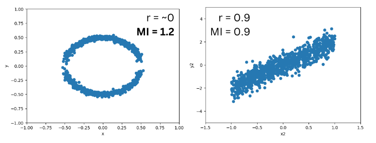
For sample data, MI detects a clear relationship between x and y while the correlation is ~0.

Summary

All in all, Mutual Information is a great alternative to Pearson correlation in certain scenarios. Try it out on your next project.

If you enjoyed this blog post, read more here, follow me on Linkedin or subscribe below.

Aaron Pickering