Aaron Pickering

Recently, I was discussing a new data set with some colleagues, the set containing several thousand patient records with several per patient. Coming from a machine learning background there were several good ideas on how to handle the data from a modelling perspective, but it surprised me to learn that no one had previously used or dealt with Hierarchical models.

I was introduced to Hierarchical models during my business and marketing consulting days and found them to be an incredibly useful technique for modelling data with categories, particularly for inference. Shortly after this conversation I gave an introduction to the topic and this intro forms the basis for the rest of this blog post.

Hierarchical modeling (also known as mixed-effects modeling or multilevel regression) is a statistical technique used to analyze data that has a hierarchical or nested structure. This type of data often occurs in studies that collect data from multiple groups or individuals, such as surveys or experiments. By using this type of model we can account for categories or groupings in the data and therefore provide more accurate and robust estimates of the relationships between variables.

Motivation

If you’re new to Hierarchical models then you might reasonably ask:

“Why bother? Machine learning models have come a long way and are incredibly powerful at teasing out complex relationships. Why use this technique?”

Therefore, I’d like to start by examining the motivation for these models and showing you why you might choose to use one.

Consider the following nested data:

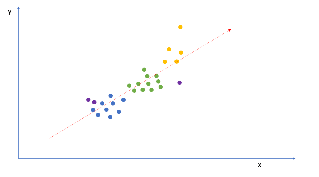
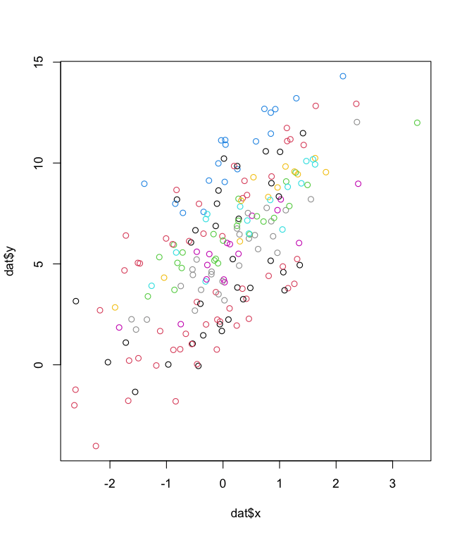
The image below shows a small (hypothetical) data set with multiple observations where each observation belongs to a group, denoted by its colour. How can we best model the relationship between x and y?

Lets start with the easiest approach and see how that looks.

Complete Pooling

The simplest approach is to just ignore the groups. If you fit a linear model with this form:

y = Bx + e

Simple univariate linear model

Then the resulting fit might look something like the image below.

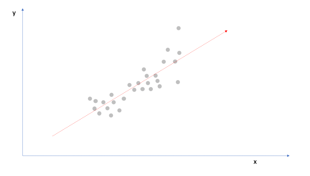
But is that really optimal for this problem? You’ve just ignored one whole variable. You may or may not be leaving out a lot of information. Let’s look again at the plot with the colour groupings. We can see that the slope for the yellow group might be a little underestimated and for purple, perhaps a little overestimated. We should be able to do better than ignoring the groups completely.

And that leads us to the next possibility.

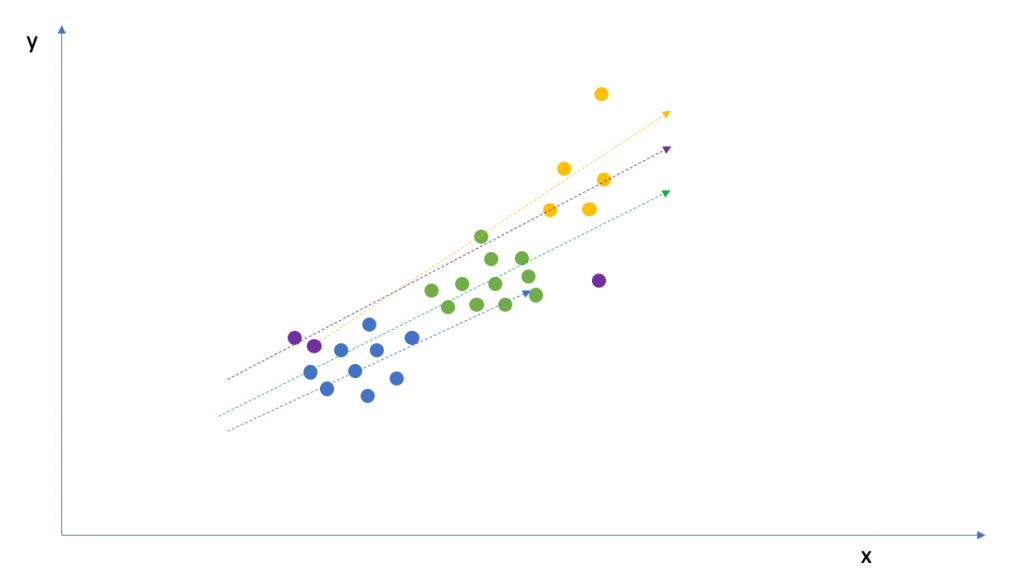
No Pooling

Lets fit each of the groups entirely separately without considering the overall structure. If we do that, we would get an individual slope per group. Importantly, as you can see, the slopes are highly susceptible to any outliers and/or small sample sizes. Consider the purple grouping – it contains only three observations and therefore our regression estimate is too flat. And the yellow grouping has a single outlier which strongly biases the slope to the positive side. This seems unrealistic.

Extreme Example

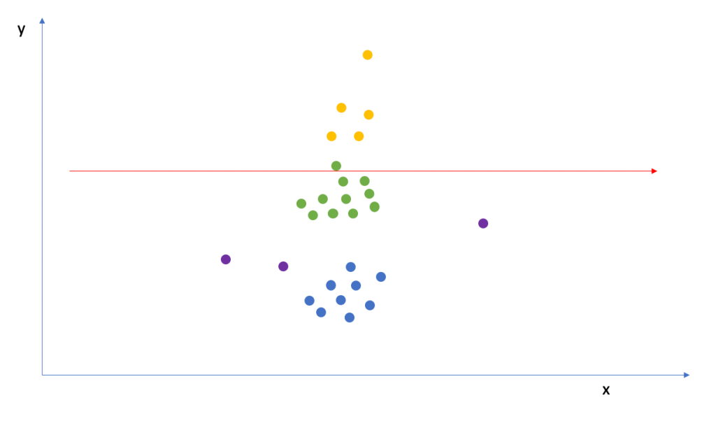
For a more serious example of where things can go wrong, consider the diagram below. In this diagram, each group has the same slope as the previous examples but they’ve been given a different intercept. You can see that they are stacked on top of each other but the slopes are the same.

If you were to use complete pooling here, you would find zero effect despite there clearly being one when taking the groups into account.

Partial Pooling

Ideally we want slopes that provide the best of both worlds, they somehow learn from the global structure but crucially, learn individual characteristics from the groups as well.

This is called partial pooling and is the key characteristic of Hierarchical or Multilevel modelling.

How it works

A typical regression model has a single error term, or depending on how you fit your model a “likelihood”. When we fit our model, we minimize the likelihood and therefore the distance between the regression and the observations.

Hierarchical models introduce another likelihood term on the parameters themselves. The assumption is that the parameters (betas, intercepts etc) are drawn from some distribution and are somewhat related.

Each parameter shouldn’t be too far away from the others, and the “force” which keeps them close is a shared parameter mean and standard deviation (assuming a Gaussian relation).

This is quite a logical assumption in many cases. For example, we would expect that many patients are quite similar to each other with perhaps a few outliers, since they are all people.

For a more formal treatment of the topic which dives into the equations, I highly recommend “Data Analysis Using Regression and Multivel/Hierarchical Models” by Gelman and Hill.

Libraries

In the next part of this article, I’ll show a simulated example to reveal some of the benefits of this approach compared to a traditional machine learning model.

However, if you’re already convinced and would like to jump straight in, the following libraries will help you get started:

Python

• Pymc / Bambi (Bayesian)
• Statsmodels (Frequentist Random Effects)

R

• BRMS (Bayesian)
• LME4 (Frequentist)

Simulated Example

For this simulated example, I created a synthetic data set with two variables, x and y. The true relationship between the variables is given by the following:

y = 2x + C + error

*where the intercept C varies by category

The “error” is a normally distributed noise term with a standard deviation of 1. See the image below showing the relationship between x and y, with the observations coloured by one of 10 different groups.

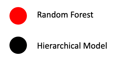
In this setup, I’ll compare the performance of a Hierarchical Bayesian Regression against a Random Forest Model (with a categorical variable included) for various data set sizes (n):

n= 30,50,100,200,500,1000,5000

For the Random Forest (RF) model, I simply feed in the group as a categorical variable without feature engineering.

How well does the Hierarchical Model perform? How well does the Random Forest perform? Can the models estimate the parameters?

Note: This simulated example favours our simple linear regression model. The results are educational and not meant to be a slight on any other model.

Results

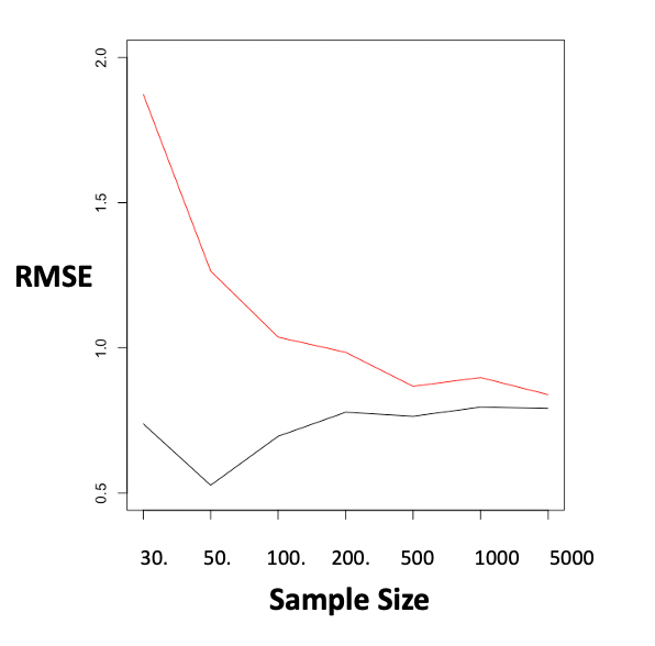
The following plot shows the predictive performance of each model as a function of the sample size used. In other words, I’ve predicted y using x and the group variable, and measured the residual errors.

At small sample sizes, the RF model is clearly outperformed. It’s error begins much higher and the gap slowly narrows to negligible numbers as the sample size increases. Food for thought.

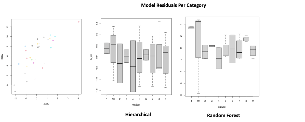
Lets also take a look at the model residuals per category. Beyond the raw error, how do the models handle the groups?

The diagram below shows the comparison for the simulation when the sample size is large. Although the total error was comparable between both models, you can see that the RF model has more variance between the group residuals and larger outliers than the Hierarchical model.

Now,lets check the residuals per group for the case when n=30. You can see that the Hierarchical model has a much “tighter” grouping of the means and significantly less group outliers than the RF. For small sample sizes, the prior encoding on the intercept makes a huge difference.

When to use a Hierarchical Model

To sum up, when should you use a Hierarchical model compared to going with a machine learning approach?

• When you have groups or categories in the data
• When the groups have some kind of logical relation that can be exploited eg. all patients have similar characteristics because they are all people
• You’re doing inference, especially at the group level
• You have a small sample size where a comparable ML model might struggle to find the interactions without explicit support
• You are especially concerned with the performance of outlying or rare observations compared to the performance of the average data point

How to do Machine Learning with Categories

One final note before I check out. In the simulation, I cheated a little bit.

Putting categorical variables straight into an ML model is not best practice. Many ML models will function sufficiently with categories but you need to do some feature engineering to make the learning process easier.

To get the best performance with ML models, use category encoding.

There are several ways of doing this including mean encoding, mean encoding with regularization and or priors, additive smoothing etc.

I actually like to think of these methods as analogous to Hierarchical learning, they work by converting the category to a numeric value based on some group value (e.g the mean) and further encoding some global group tendencies.

For more information, see this insightful Kaggle discussion.

Subscribe