Aaron Pickering

When building a model in Data Science and Machine Learning, one of the most important considerations is the target distribution. Yet, many newcomers tend to rush in, opting for RMSE or Gaussian loss without considering the nature of their data. This can lead to subpar models, especially in inference tasks where the choice of distribution significantly impacts parameter estimation.

Also, I’d like to stress that this isn’t a minor concern. A mismatched target distribution can entirely misconfigure your model. Understanding your data’s distribution is a top priority. I strongly recommend making it a habit!

In this article I’ll explore some common distributions and their applications in real world problems. In the end, you’ll have a fair idea of what each distribution looks like and when to choose them for your problem. Mostly, this knowledge was hard won, I learned them while tackling diverse problems. Through this article, I aim to smoothen your learning curve.

I won’t cover every single distribution, there are many, many variants out there. Instead, I’ll focus on roughly 90% of commonly used cases, apologies if your favorite isn’t included.

Let’s jump in!

Distribution List

Below is an overview of the distributions I’ll discuss. Click the links to head straight to the given distribution or continue reading further below.

Continuous

• Gaussian
• Uniform
• Student-t
• Gamma
• Exponential
• Log-normal
• Weibull
• Gumbel
• Beta
• Dirichlet
• Laplace
• Chi-square
• Cauchy

Discrete

• Binomial
• Bernoulli
• Poisson

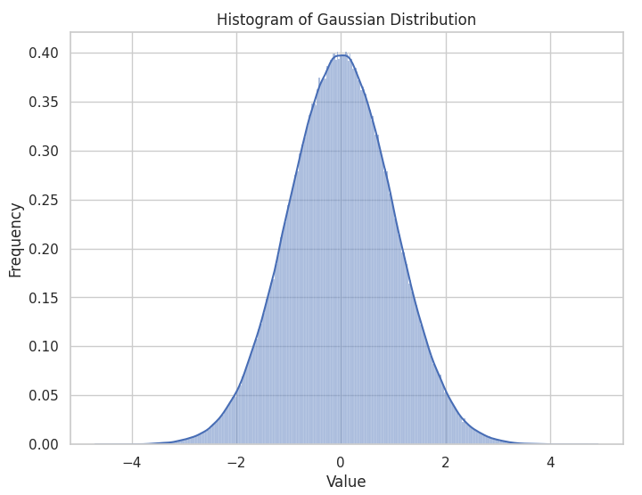
Gaussian (Normal) Distribution

The Gaussian or Normal distribution is the king of the distributions, popping up everywhere, all the time. Theres not much I can add to the topic, so for a recap check out the wiki.

The Gaussian distribution is used for many standard, continuous regression problems with positive and negative errors.

Uniform Distribution

The uniform distribution is another common distribution where all the outcomes within a given range are equally likely. Its not used much in regression but is commonly used when randomly sampling and as a ‘flat’ , uninformative prior in Bayesian setups.

Student- T Distribution

The Student-T distribution is a very common, symmetric distribution that resembles the normal distribution but has heavier tails. Move the slider on the image back and forth to compare the Student-T to the Gaussian distribution.

The Student-T distribution is very commonly used when target distribution is assumed to be normally distributed but the sample size is small. For small samples, intuitively we are unlikely to see many samples in the tail regions and for that reason, it’s hard to properly estimate the standard deviation. In these cases, the Student T distribution with fatter tails is a more robust alternative.

Its most commonly used in the ‘t-test’, a fequentist test of whether two groups have different means.

Gamma

Also known by its discrete analog, the Negative Binomial, the Gamma distribution is a 1-sided distribution with two parameters, shape and scale.

As suggested by the name, the shape parameter controls its shape. Smaller values result in distributions that peak earlier and have a longer tails, while larger values create distributions that peak later and have shorter tails. The scale parameter influences its spread.

In my experience, the Gamma distribution is the most important distributional family for regression after the Gaussian distribution. It is commonly used for measuring the time to the next event or the number of events within a certain time interval.

You can find an example of Gamma regression in my post on Heteroscedastic data.

Its also very common to see a Gamma distribution in problems where the values are bounded at zero and right skewed. This might occur, for example, in the number of sales of a product when the sales numbers are still very low. An example is given below.

Exponential Distribution

The exponential distribution is actually a specific variant of the Gamma distribution. Its your classic exponential roll-off function and can be used for modelling exponential decay.

Its used to predict the waiting time to the next effect, commonly failure or arrivals. When starting your regression model, consider the data generating process. Events be modelled by an exponential?

Common Right Skew Distributions

The next group of distributions I have grouped together for brevity. They have different use cases, but each of the distributions is bounded at zero and right skewed.

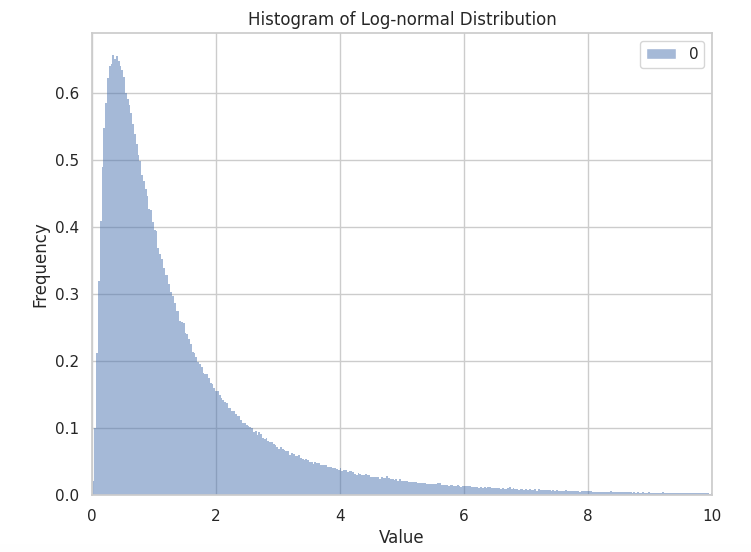
Log Normal: this distribution is used when your data is normally distributed after the application of a log transform. Its quite a common procedure and easy to test when processing the data.

Weibull Distribution: previously, I mentioned that the Gamma distribution has two parameters – shape and scale. There is a 3 parameter alternative, with 2 shape parameters. The Weibull distribution is the same as this with both shape parameters set to the same value. It’s similar to the exponential distribution with greater flexibility. This distribution is used most often to model the reliability, lifetime, and survival data in the field of engineering.

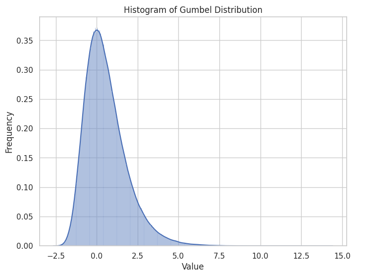
Gumbel Distribution: this distribution is used for modelling extreme values, such as the maximum value in a sample set. It’s commonly applied to analyze extreme events like floods, temperatures, or stock market fluctuations. Use this distribution when you are interested in the most extreme samples.

Log Normal, Weibull, Gumbel- click on an image to expand

Beta

The Beta distribution is a distribution defined within the range of 0 and 1. It’s often used to model variables that are constrained to this range, such as probabilities, proportions, or percentages.

Since its bounded between 0 and 1, its also used most commonly in Bayesian statistics as a prior distribution.

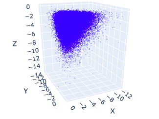
Dirichlet

The Dirichlet distribution is the multivariate form of the Beta distribution. The plot below shows an example of the 3D form (log transformed). It is used when you want to simultaneously model quantities that range between 0 and 1.

Most commonly seen in LDA.

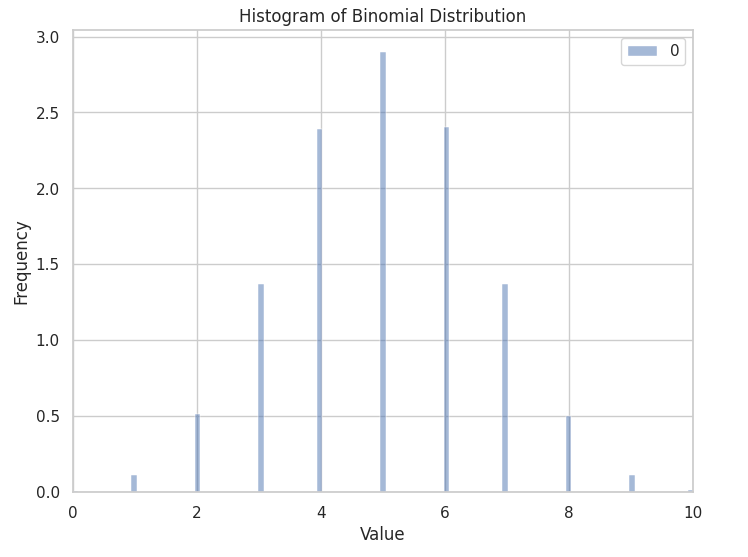
Binomial

Now we come to the discrete distributions. The Binomial distribution models the number of successful binary, given a set number of trials. For example, if you flip a coin 100 times, how many can you expect to land on heads? The value is given by a Binomial distribution.

This distribution is used often when you have multiple trials where each outcome can be either a zero or a one and you want to understand how many successes you can expect.

Bernoulli

The Bernoulli distribution is a discrete distribution, similar to the Binomial distribution but with only a single trial. What does that mean precisely?

Well, imagine that you flipped a coin, the Bernoulli distribution represents the probability that you will land on either heads or tails. If the coin is fair, the Bernoulli distribution will be 50/50 between 0 and 1.

The Bernoulli distribution is commonly used for A/B testing where user interactions are measured. For example, how many did a user click on a certain variant of a button? That process is a binary option and could be modelled via Bernoulli distribution.

Poisson

Where the Exponential distribution measured the time between events, the Poisson distribution measures the opposite. The number of events in a given time interval. It is commonly used for measuring count data e.g number of calls to a hotline, number of people in a queue etc.

The Poisson distribution is somewhat restricted because it is a one parameter distribution. The mean and variance are equal. However, the Negative Binomial (the discrete analog to the Gamma) extends the Poisson for a greater range of shapes and spreads.

Common Utility Distributions

Finally, there are three more distributions which I would like to cover. These distributions are not often used for the target distribution, rather they are used as utility functions during the modelling process. They are:

Cauchy Distribution: Fat tailed distribution, so much so that the moments are not defined (no defined mean and variance). This distribution is used in Bayesian statistics as a weakly informative prior. I understand that it’s commonly used in finance, where we want to be conservative with respect to extreme events.

Chi-Square Distribution: The chi-square distribution is a continuous distribution that arises in statistics, particularly in the context of hypothesis testing eg. Chi-Square Test.

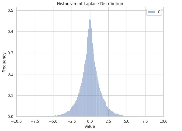
Laplace Distribution: A ‘spikier’ version of the normal distribution, this distribution is used a prior in Bayesian contexts to shrink unnecessary parameters. It is equivalent to Lasso regression.

Summary

While there are many possible distributions, this article outlines some of the most commonly used in the world of regression modelling. I hope that this article helps you select an appropriate distribution family next time you are building your model.

Subscribe

---