Aaron Pickering

For quite some time I’ve been interested in the idea of ‘time’ error, i.e. early, late, or in the time-series context, warped or unwarped. The machine learning field clings strongly to the idea using y-axis error or loss, but it’s not the only way to optimize. There is the whole error-in-variables field, for example, that includes x-axis error too. But in real life, we often talk explicitly in terms of time errors: your (probably Deutsche Bahn) train is 10 minutes late; your Amazon package gets to you a day after the expected schedule. I’ve wondered if I can use this explicitly in a regression context.

This is especially interesting to me in the case of time-series modelling. Warped series or cyclical variables with irregular phase are somewhat common in the real world, but painfully difficult to solve.

Dynamic time warping is common in the field, but it’s more of a pattern-matching tool. It doesn’t easily support regression models, inference, or forecasting. Can we build something similar that explicitly models the warping as a generative process?

Therefore, the idea behind this is simple. A given input time series x is deformed in time by some unknown or undescribed source. This deformation takes the form of slow, seemingly random expansions and contractions. What process could describe this non-stationary drift back and forth? I’ve assumed a Gaussian random walk for this time error. Not because it’s the only option, but because it’s a simple, generative way to let the series drift early and late. From there we can derive an explicit likelihood for this time error. I’m calling this “terror” (1) because of the obvious contraction and (2) because the derivation did terrorize my modest mathematical abilities.

And while fitting a random walk is infeasible (a free RW wants a value at every time step, so you get a jagged path with roughly one parameter per observation — too rough to interpret and too high-dimensional to fit usefully), it’s much more tractable to fit a piecewise-linear model approximating the path. From there, we can explicitly derive the expected likelihood between the knots: a Brownian bridge.

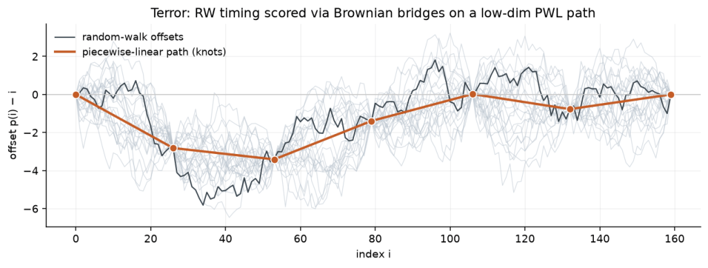
The maths for that expected Gaussian likelihood is written up here; the implementation in this repo lives in expected_likelihood_torch (PyTorch training) and expected_likelihood (JAX / Bayesian).

From there, while a bit tricky, the machinery works itself out. We have a loss function balancing y-axis and terror likelihood.

Dual likelihood:

ŷ = f(warp(x, p))

J = λ · (−log p(y | ŷ, σ_y)) − (1 − λ) · log p(p | σ_t)

So λ trades off ordinary fit (error, scale σ_y) against timing plausibility (terror, scale σ_t). At λ = 0.5 the two terms get equal weight. Toward 1 you mostly fit y; toward 0, terror takes over.

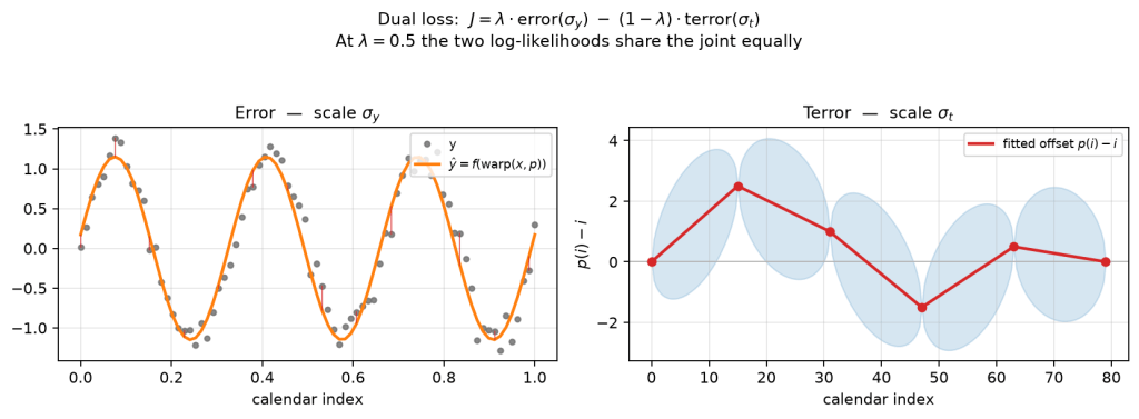
The loss function is differentiable and scalable — I’ve built it in this repo with PyTorch (and included a JAX version for Bayesian workflows). Soft-warp itself is ordinary differentiable interpolation of x at the path indices; what is specific here is scoring that path with terror and fitting it jointly with the observation model.

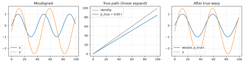
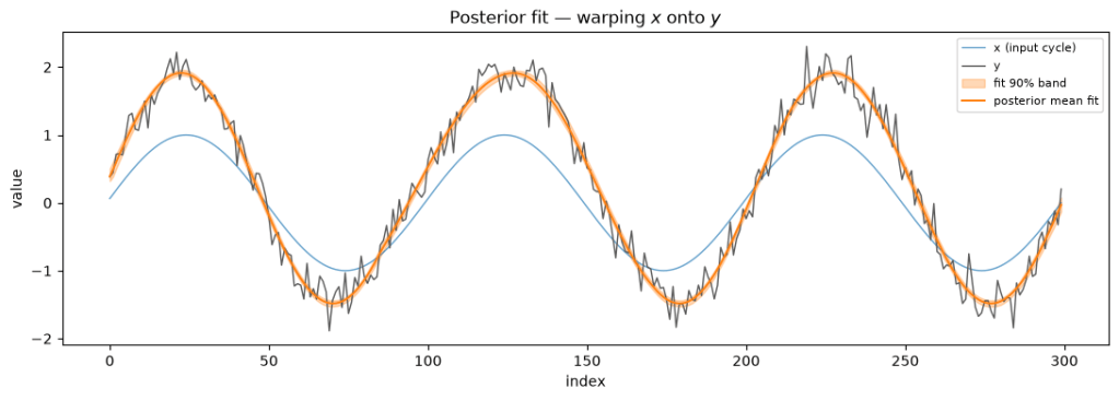
And more importantly, I think there are genuine real-life use cases for this technique. Time series with cyclical patterns (not seasonal) are very tricky to analyze with out-of-the-box tooling — and so are response shapes whose duration wanders (media carry-over, lagged physiological effects, and so on). I do not know of a single packaged tool that can do all of the following for cyclical series:

Time warping. Recover a path so a known shape lines up with the series — expansions and contractions, not just a fixed phase.

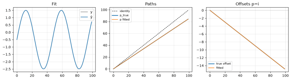
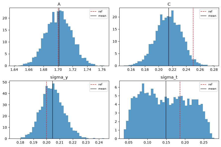
Parameterized for regression and inference. Amplitude, intercept, path knots, and both scales ((\sigma_y), (\sigma_t)) sit in one model — point estimates under the dual loss, or full posteriors when you go Bayesian.

Proper uncertainty over cycle lengths. Sample future paths under terror and measure peak-to-peak spacing — a distribution over how long the next cycle might run, not a single metronome period.

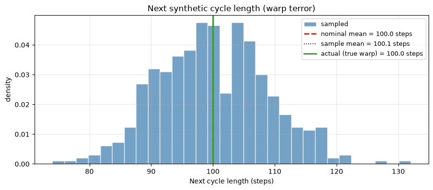
Next-cycle length under sampled warps; the dashed line is the nominal period from the prefit.

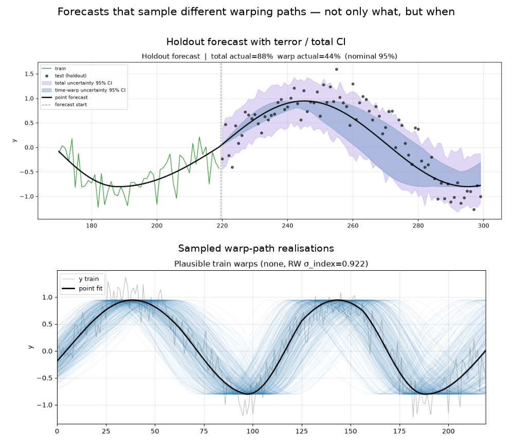
Forecasts that sample different warping paths — reflecting not only what will happen, but when. Nested CIs separate timing from observation noise; the spaghetti makes early vs late peaks concrete.

To my knowledge, there are several similar approaches that could do one or more of these things. Gaussian processes, state-space models, DTW, and DTW-style neural networks can do some of these things, but I think not all, and to my knowledge it requires highly customized, research-style approaches.

To illustrate, I have put together examples in this repository. Each one is the same dual idea — shape on x, timing on p — in a different setting.

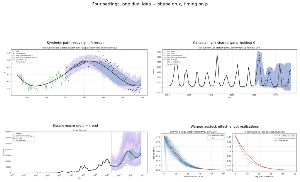
Synthetic recovery, lynx holdout, Bitcoin macro cycle, and warped adstock — one dual idea, four settings.

1) Simulated warped sinusoid.
Start with a known sine, push it through a hidden warp path, add noise, and try to recover the path and amplitude. This is the grade-school test of the method: if you cannot get the timing back when you built the truth yourself, nothing else is worth trusting. Prefit finds a rough A / C, dual fit balances residual error against terror, and you can check that the recovered path tracks the true one. Forecasts continue the path as a random walk so the bands reflect when the next peak might land, not only how high.

→ 1_Introduction_to_Warp_Regression.ipynb

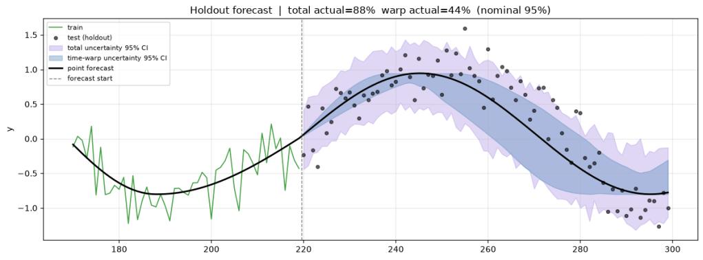
2) Canadian lynx.
The Hudson Bay trapping series is the classic irregular boom–bust cycle: a short ~10-year pulse inside a longer ~38-year envelope, with timing that stretches and compresses. We preposition those two frequencies as inputs, give each a nonlinear map for the boom peaks, and put them on one shared warp so both clocks move together. Holdout forecasts sample future warps: the MAP path looks strong early on; further out the wide terror band is the point — peaks can arrive early or late.

→ 2_Adding_complexity_Lynx_Forecast.ipynb

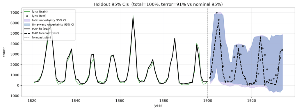
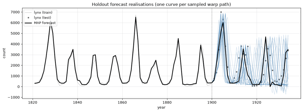
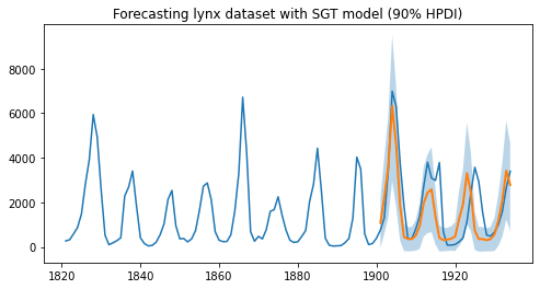
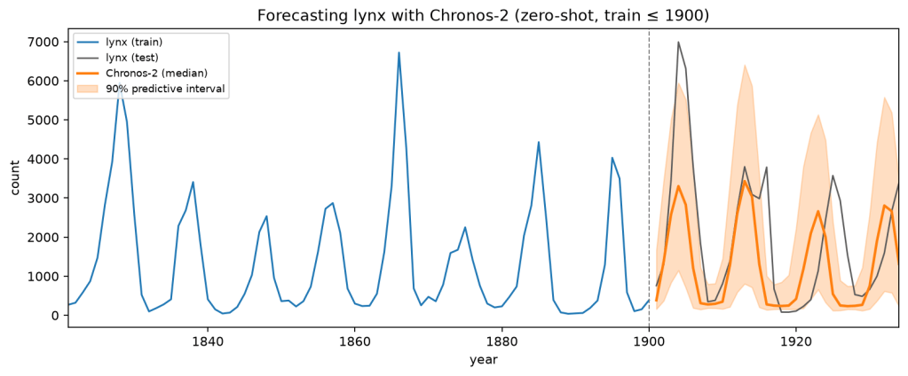
Why bother with an explicit warp? Strong baselines that treat the cycle as a fixed seasonal clock still miss the timing drift — NumPyro SGT (seasonality=38) and zero-shot Chronos-2 on the same train≤1900 split:

3) Bitcoin.
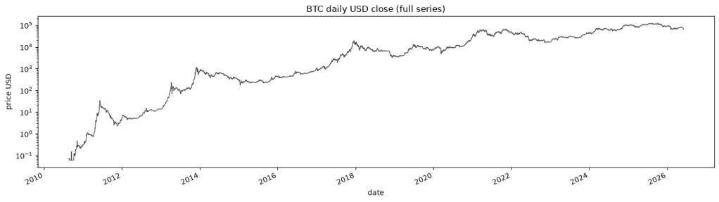
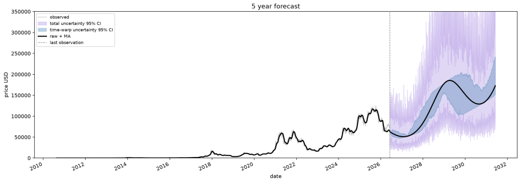
Daily log-price sits on a strong secular trend with a rough multi-year rhythm on top. The model is log-trend plus an envelope sine; the warp absorbs early and late cycle peaks instead of forcing a fixed ~4-year metronome. Out-of-sample bands again mix observation noise with terror-sampled timing, which is the point for a series where “the next top” is as much a when question as a what question.

→ 3_Bitcoin_Warp.ipynb

4) Fully Bayesian version of (1).
Same synthetic warped sinusoid and the same dual geometry, but sampled with PyMC + JAX / NumPyro instead of a point-estimate optimizer. You get posteriors on amplitude, intercept, path knots, and the two scales (σ_y, σ_t) — so path uncertainty is not a bootstrap afterthought but part of the fit. Useful when you care about credible intervals on timing, or when you want to check that the dual likelihood is a coherent Bayesian model and not only an optimization trick.

→ 4_Fully_Bayesian.ipynb

5) Marketing-mix style: warped adstock.
Classical MMM already stretches spend with an adstock (carry-over). What it usually does not do is let the duration of that effect wander as a generative timing process. Here the covariate is the already-adstocked series; pulse onsets stay fixed (p[i]=i at each spend start) so campaigns do not slide on the calendar, while the path between onsets can expand or compress. Terror is masked when spend is off, so timing is scored where the driver is active. A dual / Bayesian fit recovers the media amplitude and the warp; terror-scale random-walk bridges around the fitted path then give a distribution over how long a unit spend’s effect might last — not only how large it is.

→ 5_Marketing_Mix_Model_Warped_Effects.ipynb

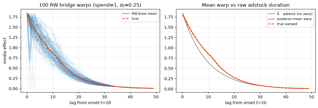
So the checklist above is not only for cycles. Anywhere a known shape is stretched in time — a media decay, a physiological response, a logistics lag — a generative warp plus terror is a way to put when into the likelihood instead of burying it in the residual.

If you want the portable building block before the full model, start with 0_Warp_Block_Basics.ipynb — a plain PyTorch WarpPath / WarpRegression recovering a known expanding warp. HTML renders of all notebooks live under examples/html/; the repo README has install and API pointers.

The working assumption throughout is simple: timing deserves its own scale, a low-dimensional path plus an expected-bridge likelihood is enough to make that trainable, and forecasts that sample when as well as what are worth the extra machinery. The examples are there to put that to the test — on a toy sine you built yourself, on lynx and Bitcoin where the clock slips, and on adstocked media where the shape is a decay rather than a cycle. If the dual loss feels like the right inductive bias for a series you care about, the code is in the repo; if not, you still have a clear story for why ordinary residual error was never going to answer the when question on its own.