Aaron Pickering

When it comes to causal stuff in industry, a common pattern I observe is that people default to the S-learner. It’s the simplest of the meta-learners: one model, treatment as a feature, done. Given how powerful and convenient these methods are, this isn’t the most egregious mistake one can make.

However, it’s important to understand the strengths and weaknesses of your models and tailor your choice to the needs of the problem. The S-learner comes with some silent disadvantages — failure modes that don’t show up in your usual cross-validation metrics, because the model is optimized to predict outcomes rather than estimate treatment effects.

Let me give you one to watch out for: regularization bias, and the way it attenuates heterogeneous treatment effects (HTEs) toward zero.

But, don’t just trust me. Let me show you via an example.

What is the S-Learner?

Very briefly: the S-learner (single-learner) fits one predictive model with the treatment variable included alongside your covariates. To estimate a treatment effect, you compare predictions under two scenarios — treatment on vs treatment off — while holding everything else fixed.

It’s appealing because you only train one model, you can reuse your favourite XGBoost hyperparameters, and it slots neatly into existing ML pipelines. I’ve used it plenty of times myself. The trouble starts when those same hyperparameters — chosen for prediction — quietly distort your causal estimates.

The Problem

In an S-learner, regularization bias arises because the model is optimized to predict outcomes, not to estimate treatment effects. Regularization settings such as strong smoothness penalties, shallow trees, aggressive pruning, or conservative learning parameters encourage simpler models that are less sensitive to small signals.

At the same time, the model tends to rely on variables that are most predictive of the outcome — which are often observed confounders that influence both treatment assignment and outcomes. As a result, the treatment variable may contribute little to the fitted model. The predicted outcomes under treatment and control end up too similar, and the estimated treatment effects are biased toward zero.

This effect is especially pronounced when confounders are strong predictors of the outcome or highly correlated with treatment assignment, since the model can achieve good predictive accuracy using the confounders alone while largely ignoring the incremental effect of treatment.

You could be forgiven for thinking the job is done if your holdout RMSE looks good. But if you look closely at the treatment effect estimates, the picture can be quite different.

The Example

Let’s start with a simulated dataset where we know the true treatment effect and can check whether the S-learner recovers it. I simulate a lot of data to test ideas like this — it’s the fastest way to build intuition before touching real production data.

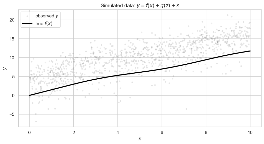
Here’s a quick look at how the data is set up:

• Treatment (x): uniform on [0, 10] — think dosage, price, or distance
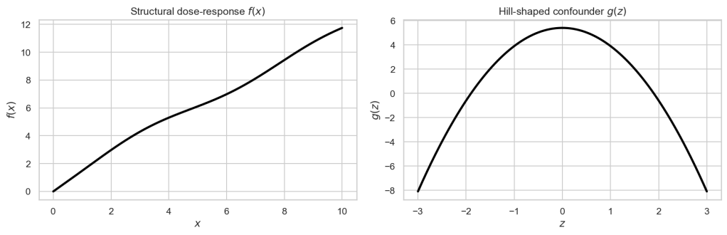
• Confounder (z): standard normal, enters through a hill-shaped function g(z)
• Outcome: y = f(x) + g(z) + ε, where f(x) is a wiggly, strictly increasing dose-response
• Noise: Gaussian with σ = 2

The S-learner fits a single XGBoost model on [x, z] to predict y. We then estimate per-unit treatment effects by bumping x by δ = 0.5 while holding z fixed at each observation’s factual value.

import numpy as np
import pandas as pd
import xgboost as xgb
from sklearn.model_selection import train_test_split
def f_structural(x):
    """Wiggly, strictly increasing dose-response in x."""
    return x + 0.5 * np.log1p(x) + 0.3 * (1.0 - np.cos(x))
def g_confound(z):
    """Hill-shaped confounder effect."""
    return 5.4 - 1.5 * z**2
rng = np.random.default_rng(42)
n = 1000
x = rng.uniform(0, 10, size=n)
z = rng.normal(0, 1, size=n)
eps = rng.normal(0, 2.0, size=n)
y = f_structural(x) + g_confound(z) + eps
df = pd.DataFrame({"x": x, "z": z, "y": y})

Here:

• f_structural is the true dose-response we want to recover
• g_confound is a hill-shaped confounder effect
• x and z are independent in this first setup (corr ≈ 0.058), so we can isolate regularization before adding correlated confounders

Minimal Regularization vs Heavy Regularization

We now learn two models for comparison:

• An XGBoost model with minimal regularization — deep trees, many estimators, light penalties
• A highly regularized XGBoost model — shallow trees, few estimators, aggressive pruning

Both models predict y reasonably well on a holdout set. If you look at the fit in isolation, you could be forgiven for thinking either spec is fine. But look at what happens when we ask causal questions.

LOW_REG_PARAMS = dict(
    max_depth=8, n_estimators=400, learning_rate=0.05,
    reg_lambda=0.01, reg_alpha=0, subsample=0.9,
)
HIGH_REG_PARAMS = dict(
    max_depth=3, n_estimators=10, learning_rate=0.25,
    min_child_weight=50, gamma=20,
)
features = ["x", "z"]
X = df[features].values
y = df["y"].values
X_tr, X_te, y_tr, y_te = train_test_split(X, y, test_size=0.2, random_state=42)
model_low = xgb.XGBRegressor(**LOW_REG_PARAMS, objective="reg:squarederror", random_state=42)
model_high = xgb.XGBRegressor(**HIGH_REG_PARAMS, objective="reg:squarederror", random_state=42)
model_low.fit(X_tr, y_tr)
model_high.fit(X_tr, y_tr)
# Per-unit treatment effect: bump x by delta, hold z fixed
delta = 0.5
x_plus = np.clip(df["x"].values + delta, 0, 10)
X0 = df[features].values
X1 = np.column_stack([x_plus, df["z"].values])
tau_hat = model_low.predict(X1) - model_low.predict(X0)

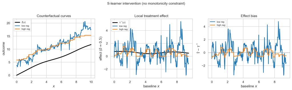
The left panel shows the fitted counterfactual curves at a reference value of z. Both models capture the general upward trend, but the highly regularized model is noticeably smoother — it has lost the wiggles in f(x).

The middle panel is where it gets interesting. The true local treatment effect τ* (black) has a clear shape. The low-reg estimate (blue) tracks it reasonably, albeit noisily. The high-reg estimate (orange) is much flatter — the HTEs have been attenuated toward zero.

On average, the true per-unit effect is 0.573. The low-reg estimate averages 0.565. The high-reg estimate collapses to 0.466.

In general, more regularization smooths treatment effects towards a flatter function. This can be good or bad depending on the situation — I’m not making any judgments on quality here, just illustrating the effect.

Confounder w Correlated with x

Now I wanted to show the impact of correlated, confounding variables. I’ve added another variable w, which is highly correlated with x. This would be similar to our price/distance relation, among others.

The extended data-generating process is:

• w = 0.85x + η
• y = f(x) + g(z) + 0.6w + ε (same f, g as before)

The learner uses x, z, w; interventions perturb x only. As a comparison, the histogram below shows treatment effect estimates with and without w in the XGBoost feature set.

# w is highly correlated with x — think price vs distance
eta = rng.normal(0, 1, size=n)
w = 0.85 * x + eta
y = f_structural(x) + g_confound(z) + 0.6 * w + eps
model_no_w = xgb.XGBRegressor(..., monotone_constraints=(1, 0))      # x, z
model_with_w = xgb.XGBRegressor(..., monotone_constraints=(1, 0, 0))   # x, z, w

Correlation between x and w is 0.927. Correlation between x and z remains near zero (0.002).

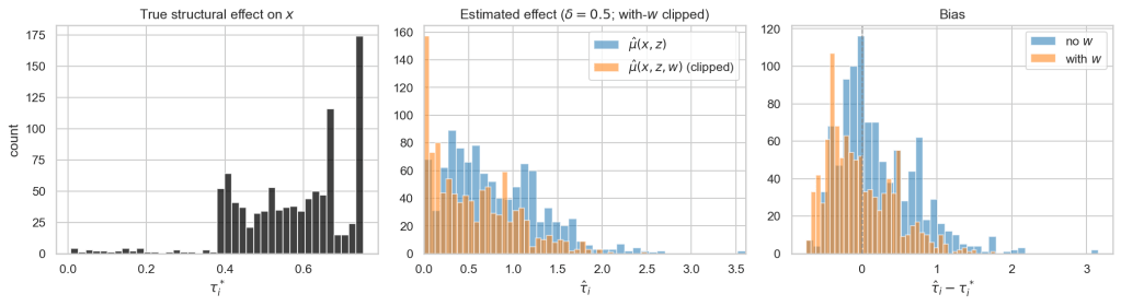
Mean true effect: 0.573. Estimated without w: 0.781. Estimated with w: 0.545.

The S-learner with the added, correlated variable w is clearly biased downwards. This occurs because the model is focused on a predictive loss, and the loss can be minimised by focusing on the other variables and ignoring the treatment. With stronger regularization hyperparameters this becomes more pronounced.

You might think adding w would help — more information! But in an S-learner, extra correlated features can steal variance from the treatment variable. The model explains the outcome through w instead of x, and the incremental treatment effect gets squeezed out.

Why the S-Learner Does This

At a high level, the mechanism is straightforward. Instead of reaching for equations, let’s break it down in plain language:

• The S-learner asks: what predicts y best? — not what is the effect of x on y?
• Regularization encourages simpler models that are less sensitive to small signals
• Confounders that strongly predict the outcome can satisfy the loss function without the model needing to use the treatment variable much
• When predicted outcomes under treatment and control are too similar, estimated effects bias toward zero

Statistician George Box once said ‘All models are wrong; some are useful’ — which applies here. The S-learner is useful for prediction. It can be misleading for causal effect estimation if you don’t watch where the regularization is pushing your estimates.

Caveats

Before you take this notebook and run with it, a few things to keep in mind:

• Simulation, not proof: this illustrates a mechanism on synthetic data where we know the truth. Real problems have messier confounding, selection, and missing variables.
• No judgment on hyperparameters: the regularization levels here are deliberately extreme to make the effect visible. Your production settings may sit somewhere in between.
• Identification still matters: even a perfectly tuned S-learner won’t save you from unobserved confounding or bad causal assumptions.

What Can You Do Instead?

There are a variety of ways to mitigate this issue:

• Audit your hyperparameters for causal impact. Try a range of regularization settings and check whether treatment effect estimates are stable — not just whether RMSE improves.
• Be careful what you put in X. Correlated confounders that strongly predict the outcome can steal signal from the treatment variable. Think carefully about whether each feature belongs in the model.
• Compare against dedicated causal methods. T-learners, X-learners, Double ML, and causal forests are all designed with treatment effect estimation in mind. I wrote about the intuition behind Double ML in a previous post if you’d like a starting point.
• Use the smell test. If your model says the treatment barely matters, or that heterogeneous effects are suspiciously flat it might not be the data lying to you. It might just be regularization and confounders quietly pulling your estimates toward zero.

Finally, choose a method whose properties match your problem! The S-learner is the default in many pipelines, but you don’t need to use it for every causal question.

Summary

In this article, I’ve shown how regularization bias in the S-learner can attenuate heterogeneous treatment effects — even when predictive performance looks fine. We walked through three scenarios:

1. High vs low regularization on a clean simulated dataset
2. The same comparison with monotonicity constraints on the treatment
3. The impact of adding a confounder highly correlated with treatment

None of this means you should never use an S-learner. It means you should understand what your hyperparameters are doing to your causal estimates, not just your RMSE. Be on the lookout for attenuated effects in your own work — especially when confounders are strong predictors of the outcome.