Aaron Pickering

Back in late 2021, I published an article entitled “Modelling stochastic time delay for regression analysis” in collaboration with Juan Orduz.

Fast forward to mid-2023, and it seems there’s still no comprehensive approach to solving this kind of problem. Admittedly, it’s niche.

But what exactly is stochastic time delay? Picture a system where the time lapse between cause and effect occurs randomly. For instance, consider a car entering a highway en route to work, its journey hindered by varying factors like traffic, obstacles, or accidents. One day, the trip might take an hour, while the next day, it could be completed in just 50 minutes.

Standard regression approaches (including machine learning) hinge on a fixed alignment between the system’s input and output, assuming a consistent delay each time. However, if this delay fluctuates, any measured effects become obfuscated.

Given my plans for a follow-up later this year, I believe revisiting and summarizing the key concepts from the original article would be beneficial. Here goes.

Challenges of Stochastic Time Delay

Consider the typical univariate regression problem where the intention is
to find the relationship between x and y. When extended to time series, a
number of time specific complexities arise. For the specific case where the input x affects the output y, with a random time delay in between, the estimated coefficients (or weights, predictions etc) are significantly attenuated. This attenuation occurs both in traditional statistical models and machine learning models, and for certain problems can be a serious limitation. The image below shows an example of stochastic time delay.

Modelling Approach

To tackle these challenges, we proposed a regression model specifically designed to handle stochastic time delay structures. Our model treats the stochastic time delay components as integral parts of the analysis rather than noise to be filtered out.

We consider the problem as analogous to the typical error-in-variables
(EIV) regression. Ordinary regression analyses (and machine learning models) define the loss function with respect to errors in the y axis only. For EIV, errors are considered in both the y-axis and the x-axis. This is
useful when there are measurement errors in the independent variable e.g. because the physical measurements have some degree of random error.

Similarly, for this problem we assume that we have errors in the y-axis and the t-axis. That is, there are random prediction errors and random errors in the time domain.

Model Specification

Given a time series x, we want to determine the functional relationship to some other target variable y ie. y = f(x(t)).

Firstly, let us take the input series x(t) and decompose it into its constituent non-zero components. So, if x(t) is a vector given by

then we decompose the vector into a matrix

where each impulse is treated separately.

Given that each non-zero impulse (row) of X(t) is affected by a random
time delay (denoted τ ), we then model:

where X(t + T) is the matrix of time shifted impulses, X(t) is the observed input, T is the set of single impulse time delays (τ ’s), 1 is the vector
(1, 1, · · · , 1) ∈ R.

The model definition represents the application of time shifts to the matrix rows and a subsequent reduction by summation over the columns.
We also assume that T is not a constant, but rather a random draw
from some discrete distribution (e.g. discrete gaussian, poisson etc). For
the discrete gaussian kernel T ∼ T(µ, σ) or for the poisson distribution
T ∼ Pois(λ). Similarly one can model the errors as ε ∼ N(µ, σε).

In order to find the best estimate of f, we would like to find
the function f which maximises the joint log-likelihood of the time-domain shifts and the prediction residuals. Specifically, we maximise:

where θ_f and θ_T represent the parameters of the model f and time shifts
T respectively. In other words, the L2 term represents likelihood of time
shifts and the L1 term represents the likelihood of the prediction residuals and we maximise these terms simultaneously.

Experiment

The following section demonstrates a simulated univariate example of
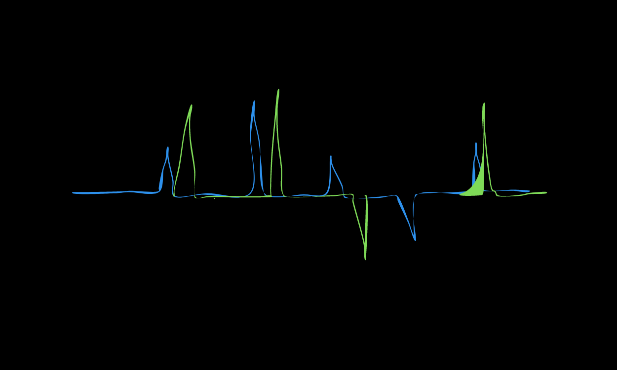
TVS Regression. Figure 2 shows the simulated time series. The full code can be found via TVS Regression on GitHub. The input signal has 20 non-zero impulses which have been drawn from the standard normal distribution. The system is ’off’ when x(t) = 0. In other words, when x(t) = 0, f(x(t)) = 0. The true shift distribution T is given by T ∼ Poisson(λ = 2). There is one value of τ for each of the 20 impulses.

The image above shows the two time series, x and y. The green line represents the real series and the orange line represents the the shifted series, corresponding to the time at which the effect occurs.

The blue line is the output y which includes a small amount of gaussian noise and an intercept. The values for the parameters were arbitrarily selected.

The relation is given by the formula below:

In essence, I’ll use a regression model to retrieve the coefficient and intercept from the equation above. The next section will show the results using this method (TVS) regression and OLS regression as a comparison.

Its an interesting exercise because you can see how biased OLS regression is in these situations, and also the benefit of our proposed solution.

Experiment Results

The table below shows the estimated effects using TVS Regression and standard OLS Regression as a comparison. TVS Regression produces results closer to the true value for the coefficient Beta and correctly estimates the random time delay noise.

The images below emphasise the comparison between TVS and OLS regression. In the top image you can see the TVS fit, in the lower left corner the OLS fit. Finally, lower right shows a scatterplot between x(t) and the estimated, adjusted x(t) and the target y.

In this case, TVS regression represents an improvement compared to OLS and allows one to properly estimate the effects.

Implications and Applications

Where can you use this model? Admittedly, it’s a relative niche technique suitable only for applications where there is stochastic delay on the input.

Where does stochastic delay occur? Some examples that come to mind from my experience:

• In marketing mix models the advertising spend is paid and logged at a fix date but the advertisement itself may actually be shown on a different, later date. This is particularly true for traditional advertising like TV and Out of Home.
• In certain medical applications, there is a delay between the drug being administered and the effect. This delay can vary semi-randomly by the characteristics of the individual, among other factors.
• Cyclical (but not periodic) time series problems e.g lynx trapping dataset.

Summary & Future Directions

This article provides a summary of the article “Modelling stochastic time delay for regression analysis”. I hope that I’ve shown some value in the technique in an understandable way. If you have any questions don’t hesitate to get in touch.

If you’d like to see an implementation, feel free to check out the repository and notebook on Github. I’m also working on a Pytorch implementation which I hope to make available in 2024.

There are several potential directions for this work. The first is to extend the method to multiple regression. I believe that the extension can be simply built on the same fundamentals discussed in this post and would allow the method to be practically useful.

Next, you may have noticed that this model is only suitable for sparse input time series with stochastic inputs. There are many cases where the inputs are not sparse e.g inputs waves where the a stochastic delay is present. This variation on the problem veers into the domain of other similar techniques such as dynamic time warping and would be very useful for e.g forecasting. I would like to tackle it in my next paper.